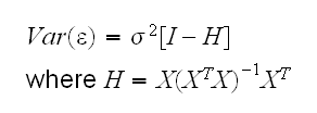
H is called the hat matrix. This is measuring the leverage of an observation because if hii is large changing yi will change the fit appreciably. The trace of H is p, the number of regressors, so "large" often means 2 or 3 times p/n.
First note that the residuals are not independent because they sum to 0 (if we fit an intercept). Their variance-covariance matrix is given by
H is called the hat matrix. This is measuring the leverage of an observation because if hii is large changing yi will change the fit appreciably. The trace of H is p, the number of regressors, so "large" often means 2 or 3 times p/n.
Example Let's illustrate these ideas using the dataset on the Scottish Hill Races. In
hills.fun(1)
we find the data matrix X, in
hills.fun(2)
the hat matrix H and with
hills.fun(3)
the observations with large leverage. There we also draw the scatterplots to see which of the observations have large leverage.
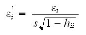
One of the consequences of having large leverage is that the corresponding observation has a smaller variance (?) One way to "fix" this is to compute the standardized residuals:
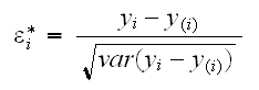
Another problem for the residuals is if one observation has an error which is very large because then the estimate of σ will be too large as well, and this makes all the standardized residuals to small. A possible way to proceed is to find the studentized residuals as follows:
1) fit the model but without the use of the ith observation, then use the model to find the prediction y(i) for yi.
2) The studentized residuals are
An easy way to find the studentized residuals is using the formula
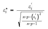
Studentized residuals are sometimes also called jackknifed residuals.
hills.fun(5)
draws the residual vs. fits plots and
hills.fun(6)
the normal plots using the three residuals
In
hills.fun(7)
we again draw the stud. residual vs. fits plot, and identify two outliers, Bens of Jura and Knock Hill. Bens of Jura has a high leverage and a high studentized residual. Knock Hill has a very high residual but not a large leverage. Predicting the time for the Knock Hill race from the model using
hill.fun(8)
we find predict(fit)=13.5, more than an hour less than the time in the dataset. This could possibly be a missprint.
The leverage discussed above has a major drawback as a measure of "outlierness": it ignores the response y. In general we are most concerned with observations whose removal will change the fitted model dramatically. How can we identify such "influential" observations? One measure of influence is Cook's distance. It uses the leave-one-out cross-validation idea already discussed above for the studentized residuals. Say we eliminate the ith observation and fit the model using the remaining i-1 observations. Let's call the resulting vector of parameter estimates  (i). As always denote the the estimtor when we use all the data . Then Cook's distance is defined by
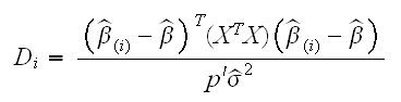
As a rule of thumb values of Di larger than 1 should be considered for removal. A plot of Cook's distance is drawn in
hills.fun(9)
What happens if we eliminate Knock Hill and/or Bens of Jura from the analysis?
hills.fun(10)
shows that the removal of Knock Hills does not change things much wheras the removal of Bens of Jura does.
One undesirable feature of the fit is the (statistically significantly) negative intercept (?). Of course we could set it equal to 0 by ourselves but it would still be nicer if the model did this automatically.
Example nNext we have a look at a dataset describing the relationship between body weight and brain weight of mammals. In
mammals.fun(1)
we draw the scatterplot of Brain weight by Body weight. This graph is hard to read because most of the space is taken up by just two observations, identified as Asian and African Elephants. The problem here is that the distributions of both body and brain are scewed to the right, as can be seen by adding the boxplos
mammals.fun(2)
This kind of problem can often be fixed using a log transform. In
mammals.fun(3)
we draw the corresponding boxplots and scatterplot, and we see that this indeed solves the problem.
What does this transform do?
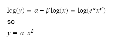
and we see that this fits a power model.
In
mammals.fun(4)
we do the fit and study the diagnostic plots. Observation #32 appears as unusual in some of the diagnostic plots, and we find it to belong to the species "Human"
Example Let's study the dataset Medieval Churches.
attach(churches)
addbox(Perimeter,Area)
shows a strong relationship, but one that is clearly not linear. We also have some skewdness to the right again and a possibility of unequal variance. As before we can try and remedy that via a transformation, for example using logs:
addbox(log(Perimeter),log(Area))
This seems to do an ok job. But is there a way to do better, maybe in some sense find an "optimal" transformation? For this let's consider the Box & Cox transform
The routine boxcox draws the profile likelihood curve together with a 95% confidence interval. Basically any value of λ in this interval yields a transformation close to optimal. For our dataset this is done by
churches.fun(3)
It shows that values between 0.45 and 0.8 are acceptable. The "nicest" value in this interval is 0.5, corresponding to the square root transform of Area. Notice that it sufficient to use √(Area) instead of (Area0.5-1)/0.5.
churches.fun(4)
fits the corresponding model and studies the diagnostic plots, and in
churches.fun(5)
we draw the fitted line plot. Note that the resulting model still has a hint of unequal variance.