Nonlinear Parametric Models

Example Consider the dataset Lobster. In

lobster.fun(1)

we draw the scatterplot of Length by Time and see that the relationship is highly nonlinear, which of course is to be expected.
We have already seen a number of strategies we could use to fit this dataset:

• a polynomial model, see

lobster.fun(2,deg)

• a loess fit, see

lobster.fun(3)

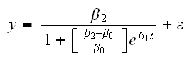
Often, though, there are already standard models for certain types of relationships that have been used successfully in the past. For example, if our model is supposed to describe radioactive decay it makes good sense to use a model of the form y=αe^-βt+ε, a model suggested from Physics. Our dataset also describes a specific kind of relationship, a growth model, and such a relationship is often modeled using the equation

where

β₀ is the expected value of y at time t=0
β₁ is a measure of the growth rate, and
β₂ is the expected limit of y as t∞

This is often called the logistic or autocatalytic model

How do we fit such a model, that is find "optimal" values of β₀, β₁ and β₂? Sometimes it is possible use transformations to "linearize" the model, for example we have of course log(y)=log(α)-βt for the radioactive decay model. This is not possible, though, for the logistic model, so we have to find a different solution.

Previously we have always used the method of least squares to estimate the parameters in our models, that is we minimized the "figure of merit"

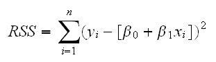
We can extend this easily to our problem by minimizing

where f is the function describing the model and β is the vector of parameters.

For the linear model minimizing RSS is a simple exercise in Calculus. Unfortunately in more complicated situations minimizing RSS can no longer be done explicitely but has to be done numerically. In R we have a function built in to do it for use, namely nls. It is used in

lobster.fun(4)

to fit the growth model to the lobster data.

By default nls uses the Newton-Raphson algorithm to find the minimum of RSS.

The hardest part for using the nls function is finding a good starting point x⁰. (β₀=100? β₂=500?)

As an alternative to using least squares we could also have used maximum likelihood.

Fitting Splines with Unknown Knots

Let's return to the artificial example we used to illustrate splines. There we assumed that we know that the knot is at x_k=5.0. Say we did not know where the knot is and wanted to include it as a parameter in our model. Now the model is no longer linearizable, but we could again use nls. This is implemented in

splines.fun(2)

Note that on occasion the minimizer fails to converge, not unusual in a problem in 8 dimensions.