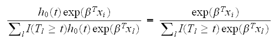
which does not depend on the baseline hazard. The partial likelihood is the product over all such terms over all observed deaths, and contains most of the information about β.
A nonparametric approach to survival data was first introduced by Cox in 1972. Here we model the hazard function h as follows: there is a baseline hazard h0(t) which is modified multiplicatifely by covariates, so the hazard function for any individual case is h(t) = h0(t)exp(βTx), and the interest is mainly in β.
The vector β is estimated via partial likelihood. Suppose a death occurs at time tj. Then conditionally on this event the probability that case i died is
which does not depend on the baseline hazard. The partial likelihood is the product over all such terms over all observed deaths, and contains most of the information about β.
Example In
leuk.fun(11)
we use the function coxph do find the Cox proportional hazard model for the leukemia data. We also use the resulting model to plot the survival curve, together with the corresponding parametric etimates.
Example Next we have a look at the Lung Cancer dataset. In
lung.fun(1)
we have a look at the summary statistics of the data. One thing to notice is that several variables have missing values, coded as NA.
If we want to have a look at some graphics relating the covariates to time we have to deal with the censoring. One way is to remove all the censored cases, which we do in
lung.fun(2)
By default both boxplot and plot remove all missing values from the dataset.
Next we want to fit the Cox proportional hazards model, but there are two issues we need to deal with:
• what to do with the missing values? we remove them from the dataset using na.action=na.omit
• in this experiment sex was a stratification variable. We can include this fact in our model by using strata(sex) instead of just sex. This allows for nonproportional hazards.
The corresponding model is fit in
lung.fun(3)
Notice the three hypothesis tests at the bottom. They do the job of the F-test in regression, namely testing whether all the variables together are useful for predicting time. Hear clearly they are.
Checking the individual covariates we see that age and meal.cal are not significant. In
lung.fun(4)
we refit without them. One unfortunate consequence of the missing values is that we can not compare the two models directly.
Next we want to try and assess whether this model is appropriate. In regression we use the residual vs. fits plot for this purpose. Here we have something similar. There are actually several kinds of residuals in a survival analysis, we will use what are called the martingale residuals. The plots are the residuals with the variable of interest vs. the residuals without the variable of interest. Again we need to deal with the missing values, and we remove them from the dataset. Finally we add a loess curve to the graphs. All of this is done in
lung.fun(5)
All of the relationships look reasonably linear.
In regression analysis we worried about observations with a large influence (outliers?) An analog of Cook's distance plot is drawn in
lung.fun(6)
where we use a different kind of residuals using type="dfbetas" in the call to resid(fit). The largest change in coefficients is 0.6 standard errors of the coefficient of ph.karno. Since ph.karno is only marginally significant (p-value=0.093) this is no cause for concern.
Finally we can have a look whether the assumption of proportional hazards is justified. For this we use the cox.zph function. This plots the rescaled Shoenfeld residuals. A flat appearance indicates that the assumption is ok. The correspnding object carries out hypothesis tests for a significant slope in the scatterplots, which support our assessment.
lung.fun(7)