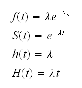
• Exponential distribution:
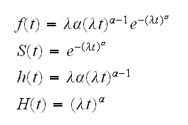
• Weibull distribution:
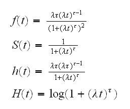
• Log-Logistic distribution:
as well as the log-normal and the gamma distribution.
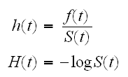
 (0,∞) and T has a continuous distribution F with density f. In survival analysis several functions are of common interest:
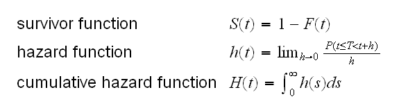
Here are some examples for commonly used lifetime distributions:
• Exponential distribution:
• Weibull distribution:
• Log-Logistic distribution:
as well as the log-normal and the gamma distribution.
Example consider the Leukemia dataset. The most commonly used estimator for the distribution function F is the empirical distribution function, and so we could use that to estimate S. This is done in
leuk.fun(1)
for the two test results separately.
The most distinctive feature of survival analysis is censoring. Say we are testing a new treatment for late-stage AIDS. At the beginning of the study we select 100 AIDS patients and begin treatment. After 1 year we wish to study the effectiveness of the new treatment. At that time 47 of the patients have died, and for them we know the number of days until death. For the other 53 patients we know that they have survived 365 days but we don't know how much longer they will live. How do we use all the available information?
Censoring comes in a number of different forms:
• right censoring: here "case i" leaves the trial at time Ci, and we either know Ti if Ti≤Ci, or that Ti>Ci.
• we have random censoring if Ti and Ci are independent.
• type I censoring is when the censoring times are fixed in advance, for example by the end of the clinical trial.
• type II censoring is when the the experiment is terminated after a fixed number of failures.
In R we code the data as a pair (ti, di) where ti is the observed survival time and di=0 if the observation is censored, di=1 if a "death" is observed.
urvival data is often presented using a + for the censored observations, for example 35, 67+, 85+, 93, 101, etc.
Let t1*<t2*<..<tm* be the m distinct survival times. Let Yi(s) be an indicator function, which is 1 if person i is still at risk (that is alive) at time s and 0 otherwise, that is Yi(s)=I(0,ti*)(s).
Then the number of patients at risk at time s is r(s)=∑Yi(s). We can similarly define d(s) as the number of deaths occuring at time s.
There is also a modern approach to survival data based on stochastic processes, especially martingales and counting processes. In this setup one considers the counting process Ni(t) associated with the ith subject, so Ni(t) changes by 1 at each observed event ( for example, a vist to the doctor, a heart attack, a death etc).
How can we estimate the survivor curve in the presence of censoring? One of the most commonly used estimators is the Kaplan-Meier estimator:
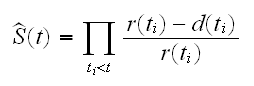
In R this is computed with the function survfit. It uses as its argument a "survival" object which in turn is generated using the Surv function. We do this for the Leukemia data in
leuk.fun(2)
have a look at the resulting fit object and what it's parts are.
leuk.fun(3)
plots the estimated survival curves and compares them to those using the empirical distribution function.
Another popular estimator implemented in R is the following:
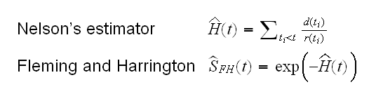
leuk.fun(4)
plots the two estimates side by side.
Example Let's have a look at the dataset Gehan. In
gehan.fun(1)
we draw the estimators for the survival curves.
Is there a difference between the remission times of the two groups? We use survdiff in
gehan.fun(2)
and see that indeed there is.
Confidence intervals for the survival curve are automatically computed by the survfit function. By default it finds intervals of the form S±1.96se(S). Other options are:
• conf.type="log": exp(log(S)±1.96se(H))
• conf.type="log-log": exp(-exp(log(-log(S)±1.96se(log(H)))
One advantage of log-log is that the limits are always in (0,1).
gehan.fun(3)
finds 90% confidence intervals based on these three methods for t=10 in the 6-MP group.
An important question for new patients is of course the average survival time. As always "average" can be computed in different ways. R uses the median and the estimate is part of the output for a survfit object, see
gehan.fun(4)
Sometimes it is possible to fit a parametric curve via generalized linear models to the survival curve. Say we wish to fit an exponential model, and suppose we have a covariate vector x for each case. Say λi is the rate of the exponential for case i. Then we can connect the rate to the covariates via the model λi=βTx. This might on occasion be negative, and it is often better to use log(λi)=βTx
Example Let's see whether the Leukemia data can be modeled in this way. First we have a look at the relationship of time and its covariates:
leuk.fun(5)
The relationships do not appear to be linear, and we fix this by using a log transform on time and wbc.
What model might be appropriate for this dataset? For the exponential model we have -logS(t)=H(t)=lt, so if we plot -logS(t) vs t we should see a linear relationship:
leuk.fun(6)
In
leuk.fun(7)
we fit this model via glm. Another way to fit the same model is using the routine survreg written by Terry Therneau, as done in
leuk.fun(8)
As an alternative we might consider fitting a Weibull distribution, which is a generalization of the exponential. We have the following:
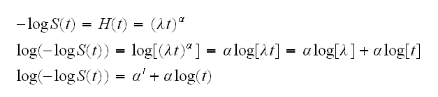
and so in this case a plot of log(-log(S)) vs. log(t) should be linear. This plot is done in
leuk.fun(9)
Notice that the Weibull distribution is the default model of survreg. In the output we see that the p-value of log(scale) is 0.77, so log(α) is statistically consistent with 0, or α with 1, which means the Weibull distribution does not give a stat. sign. better fit than the exponential.
Example A similar analysis is done in fsgehan.fun(5) to gehan.fun(7), where we find that the exponential model fits well and that the covariate pairs does not add significantly in the model.