Robust Regression

Example Consider the dataset on the expenditure on alcohol and tobacco. In

alcohol.fun(1)

we draw the scatterplot and see that there is a serious outlier, identified as Northern Ireland. In

alcohol.fun(2)

we add the least squares regession lines with and without Northern Ireland, and we see that they are very different. How should we preceed with this analysis?

First we should always try and understand why an observation is an outlier. In this case an educated guess is fairly simple (?). But then we need to decide how to proceed.

One option is of course to remove the observation from the dataset. In this case, though, this means removing 9% of the data. Do we have any other options?

R has a number of robust regression methods implemented:

Least Median of Squares (LMS)

In least squares regression we find the parameter estimates by

min{∑ (y_i-β'x_i)²}

Part of the reason least squares regrssion is so sensitive to outliers is the square in this formula. So Rousseeuw suggested to instead use

min{ Median(y_i-β'x_i)²}

This is called least median of squares (LMS) regression and is implemented in R by the function lmsreg. To help with certain problems Rousseeuw later suggested a variation of this method using

min{∑_I|y_i-β'x_i|²_(i)}

where the sum is taken over the indexset I of the smallest residuals. This method is called LTS and is implemented in R in ltsreg and is preferred over lmsreg. In

alcohol.fun(3)

we add the LTS line to the plot and we see that it is somewhat between the two "extreme" lines, and a little closer to the one without Northern Ireland.

Huber's M estimator

Let's first have a look at a very simple problem, estimating a location parameter μ. So say we have data X₁, .., X_n iid with some density f and we want to estimate μ=EX₁. Using the method of least squares means minimizing the expression ∑(X_i-a)², which of course leads to the sample mean. It is highly sensitive to outliers because of the use of the square, though. Alternatively we could use as our "figure of merit" ∑|X_i-a|. The a that minimizes this expression is the median, which is highly robust but unfortunately not very efficient. Huber (1964) proposed a compromize between these two, namely to minimize ∑r(X_i-a) where ρ is given by

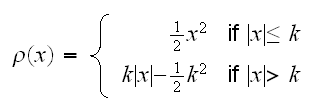
The function ρ(x) behaves like x² for "small" x (|x|≤k) and like |x| for large x (if |x|>k). It is easy to show that ρ is differentiable so the minimization above can be done numerically. The constant k is a tuning parameter, with k=∞ yielding mean square and small k's leading to median-like estimators.
Huber also studied other functions for ρ. Together they are referred to as Huber's M-estimators, for "maximum-likelihood-type" estimators. These also exist for the regression problem, and are implemented in the function rlm in R. In

alcohol.fun(4)

we add this line to our plot as well. We can supply the tuning parameter k and we see that for k>3.2 this line is the same as the least squares regression line. For k=0.1, say, we almost get the line based on medians. The default is k=1.345.

Let's study the performance of these methods. For this we need to simulate data with outliers. There are of course a great many ways in which an observation can be an outlier. We will consider two:

1) with respect to y. Here we generate data as follows: x₁, .., x_n ~ N(0,1). Then y_i=x_i+N(0,0.25) for i=1,..,n-1 and y_n=x_i+N(7,2)
2) with respect to x. Here we generate data as follows: x₁, .., x_n-1 ~ N(0,1), x_n~N(10,3). Then y=x+N(0,0.25)

Examples of these are illustrated in

robust.sim(1,1)

and

robust.sim(1,2)

, together with four fitted lines:

• least squares (black)
• LTS (red).
• Huber, default k (green)
• Huber, small k (blue)

How do we measure the effect of the outlier? In case 1) it appears that in least squares regression the coefficients are wrong. We check that doing a simulation in

robust.sim(2,B=100)

The result is shown in

robust.sim(2,1)

for β₀ the least squares regression is biased abwards whereas the three robust methods work well, and for β₁ the least squares regression has a much larger variance than the other three methods.

How about the second type of outlier? In

robust.sim(2,2)

we draw the corresponding boxplots and we see that here least squares actually does quite well, it seems LTS does worse than the others.

How do these outliers effect prediction? We run a small simulations study, finding 95% confidence intervals for the mean response at x=0.2. (Note we can not use ltsreg because its predict method does not return the standard error or confidence intervals). Here are the results:

Type	lm	rlm	rlm(k=0.1)
1	99.1	81.8	99.1
2	94.7	81.4	94.7