Regression Trees

Tree-based methods partition the feature space into a set of rectangles, and then fit a simple model (for example a constant) in each one. They are conceptually simple yet powerful. They have been in use in many fields in the past, for example in Biology. (Animal or Vegetable?) In Statistics they became popular with the work of Breiman et al. in the 1980's

As an illustration consider a continuous reponse variable y and two continuous predictors X₁ and X₂, each with values in [0,1]. A partition of the feature space is given in

tree.ill(1)

This is a prefectly legitimate partition but it has the problem that it is very difficult to describe. Instead we will restrict ourselves to the use of recursive binary partitions like the on shown in

tree.ill(2)

Such a tree is very easy to describe using a tree diagram, see

tree.ill(3)

In this diagram each split is called a node. If it does not have a further split it is called a terminal node.
The corresponding regression model predicts Y with a constant c_m in Region R_m, that is

How to grow a tree

Say our data consists of p "inputs" and a response for each of n observations, that is (x_i,y_i) for i=1,..,n, with x_i=(x_i1,..,x_ip). The algorithm needs to automatically decide on the splitting variables and split points, and also what topology (or shape) the tree should have. Suppose that first we partition into M regions R₁, .., R_m, and we model the response as a constant in each region:

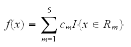
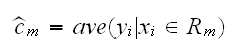
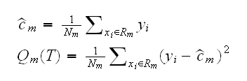
if we adopt as our criterion minimization of the sum of squares ∑(y_i-f(x_i)², it is easy to show that the best constants c_m are just the mean values of y's with corresponding x's in R_m:

Now finding the best binary partition in terms of minimum sum of squares is generally not possible for computational reasons, so we proceed as follows: Starting with all the data, consider a splitting variable j and split point s, and define the pair of half-planes

Then we seek the splitting variable j and split point s which are optimal, which for any choice of j and s is done by

For each splitting variable, the determination of the split point s can be done very quickly and so by scanning through all of the inputs we can find the best pair (j,s).

Having found the best split we partition the data into the two resulting regions and repeat the splitting process on each of the two regions. Then this process is repeated.

How large should a tree grow? Clearly without any "stopping rule" the tree will grow until each observation has its own region, which would amount to overfitting. The size of the tree is in fact a tuning parameter such as span for loess, governing the bias-variance tradeoff.

The most common strategy is to grow a large tree T₀, stopping only when some minimum node size (say 5) is reached. Then this large tree is pruned (made smaller) using cost-complexity pruning:

Say T₁ is a sub-tree of T₀, that is T₁ can be obtained by pruning branches off T₀. Let |T| be the number of terminal nodes in T and index the terminal nodes by 1,..,m. Let

then we define the cost-complexity criterion

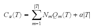
the idea is to find, for each α, the subtree T_α to minimize C_α(T). The tuning parameter α governs the trade-off between the size of the tree and the goodness-of-fit to the data. If α=0 the solution is the full tree T₀, and for larger values of α the tree becomes smaller. Methods to choose an "optimal" α automatically are known, for example cross-validation.

Examples

In R we have the routine rpart (recursive partitioning) to fit tree models.

Let's begin with an artificial example. In

tree.ill(3)

we draw the tree for a simple model, and in

tree.ill(4)

we generate 1000 observations as according to that model, fit the regression tree and plot the fitted model. Clearly the regression tree "recovers" the model very well.

tree.ill(5)

plots z vs. x and z vs. y. Looking at these graphs it is not clear how one would fit a standard model to this dataset.

Example As a first real example let's return to the kyphosis dataset. In

kyphosis.fun(9)

we fit a regression tree to the data. The best way to look at the resulting tree is with plot(fit) (followed by text(fit) for the labels).

Example consider the US temperature dataset. In

ustemp1.fun(8)

we fit a tree and look at the "fitted plot".

Example In

solder.fun(7)

we consider a regression tree for the solder data

ExampleI n

airpollution.fun(2)

we do the regression tree for the air pollution data. How does this model compare with a "standard" fit? In

airpollution.fun(3)

we find the residual sum of squares for the tree and for the model based on lm, which is a little bit smaller.