and if the errors have a normal distribution we can find an interval estimate based on normal theory. This is often called a confidence interval.
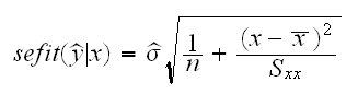
• Say we want to estimate the mean response for a given value of x, that is μ(x*) = E[y*] = f(x*). It can be shown that the standard error is given by
and if the errors have a normal distribution we can find an interval estimate based on normal theory. This is often called a confidence interval.
• Say we want to estimate the y* for a given x=x*. Now the standard error is given by
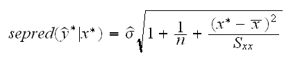
Intervals based on this error are called prediction intervals.
Example let's consider one of the truly famous datasets in Statistics regarding the eruptions of the Old Faithful guyser.
In
faithful.fun(1)
we look at the scatterplot of eruptions by time. There is a clear linear relationship between the length of the eruption and the waiting time until the next one. In
faithful.fun(2)
we fit a linear model and check the assumptions, which appear just fine. In
faithful.fun(3)
we draw the fitted line plot.
In this problem clearly it is of interest to predict the waiting time for one observation rather than the mean response. Say we wish to predict the time until the next eruption if the last one took 4.5 minutes. In
faithful.fun(4)
we find the point estimate to be 81.8 and the 95% prediction interval is (70.1, 93.4) minutes.
The interval is of the form y*±zα/2sepred, and we use this in reverse to find the prediction error to be 5.96 minutes.
Example In
highway.fun(9)
we find the 90% confidence interval for the mean accident rate of roads that are "average" (in the sense of the median) using a model based on len, slim and acpt.
Predicting for an x value not to different from x values in the dataset is usually called interpolation whereas predicting for an x value well outside the range of observed x values is called extrapolation. Extrapolation in general is much less reliable than interpolation because we have to make the assumption that the observed relationship continuous to hold there.
Example consider the fish storage data. In
fish.fun(1)
we draw the scatterplot and find a strong linear relationship. In
fish.fun(2)
we run the regression and check the assumptions, all of which are fine. In
fish.fun(3)
we draw the fitted line plot.
In
fish.fun(4)
we use the linear model to find the 95% prediction intervals for fish that were put in storage after 5.5 hours and 20.5 hours, respectively. These two intervals are very different, though: the one for 5.5 hours seems quite fine whereas the one with 20.5 hours is almost certainly nonsense. In
fish.fun(5)
we show why.
Example Let's go back to the Old Faithful dataset, and assume the park rangers want to post a table that lists the 95% prediction intervals for the waiting times if the last eruption lasted 1,2, 3, 4 or 5 minutes. In
faithful.fun(6)
we show this table.
What is wrong with this? The problem is that each interval individually is a 95% prediction interval but the collection of 5 intervals is not. That is if we kept track of all the eruptions during a day and how often the table gave the correct predition we would find the table to be wrong much more often then 5%. This is illustrated in the routine predict.sim. Here we use a simple model (y=10+3x+N(0,3)) and run a simulation to study the true coverage rate. In
predict.sim(1)
we just predict for one x value, and we see that the true coverage rate at the nominal 90% level is in fact around 90%. In
predict.sim(2,1,10)
we draw the 90% prediction intervals together with the new observations, using red if the interval does not contain the y value. As we see most pictures contain at least one "wrong" interval. In
predict.sim(3,100,10)
we run the simulation for 10 points (based on 100 runs) and find the true overall coverage rate to be just about 30%. In
predict.sim(4)
we see the results of 10 studies and based 1000 runs each.
What is the problem here? Let's assume we have p intervals I1,..,Ip and use them as prediction intervals for new observations y1*, .., yp*. Each interval individually is a 100(1-α)% prediction interval. Then their simultaneous coverage is
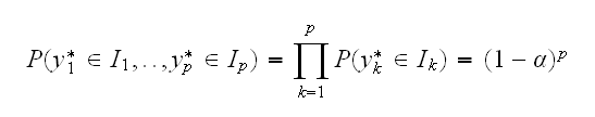
if we assume independence (?). In
predict.sim(5)
we again print the true coverage rates together with the theoretical one from this calculation, and we find quite a good fit.
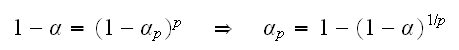
What can we do to achieve an overall coverage of 100(1-α)%? Bonferroni's method is based on the calculation above:
In
predict.sim(6)
we run the simulation again, with these adjusted confidence levels. The results are printed in
predict.sim(7)
As we see, here this works very nicely.
How about confidence intervals? In
predict.sim(9)
we have the results of a simulation study like the one above, but for confidence intervals. We see that here it does not work as well, Bonferroni's method overcompensates and yields confidence intervals that are too conservative, that is they are to long.
What is the difference between the two? Independence! Because prediction intervals are for new y*'s there is a degree of independence between the intervals, whereas the confidence intervals are quite dependent.