Problems with just one predictor are sometimes called simple linear regression problems whereas problems with 2 or more predictors are called mutiple regression problems.
Example Let's have a look at a dataset for Highway accidents.
As a first look we might study the distribution of each variable separately, to see whether there are any that clearly don't have a normal distribution and whether there are any outliers. Note that several of the predictors (fai, pa and ma) are dummy variables, so for them those questions don't arise. This is is done in
highway.fun(1)
Although some of the variables appear to be somewhat skewed (for example itg) none is bad enough to need immediate attention.
Next we can have a look at some summary statistics such as means and standard deviations as well as the correlations. This is done in
highway.fun(2)
Checking the correlations between predictors is important because if some of them are highly correlated (collinearity) then regression becomes suspect, In the extreme case of perfectly correlated predictors (for example temperature measued in °C and in °F) it becomes impossible. In our case the largest correlation is 90% (adt and itg), which is usually ok.
Next we run a linear regression of rate on all the other predictors, in
highway.fun(3)
We see that one observation(#25) is rather unusual (with a Cook's distance of almost 1) and one might consider removing it, although we will not do so here.
Note that none of the predictors is stat. significant by itself (according to the t-tests) but the model as a whole is ( the F-test)
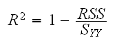
Looking at the fitted model we see that R2=76%. R2 is called the coefficient of determination and is an overall measure of how well the model explains the response, with an R2 close to 1 indicating a good model. It is defined as
In a simple regression problem we have R2=(r)2*100%, where r is Pearson's correlation coefficient.
Whether R2=76% is good or not depends on the subject matter, in some fields (like Chemistry) it would be considered horrible whereas in other fields (say Social Sciences) it might be quite excellent.
One major task in such a problem is to find a parsimoneous model, that is a model with as few predictors as possible while still retaining a model with a good fit. The difficulty here is that removing any of the predictors will always result in a worse fit, for example as measured by R2. In
highway.fun(4)
we illustrated this by dropping one variable at a time and finding the corresponding R2. The reason for this is obvious: say we have a model
y=5.6+7.8x
with R2=80%. Now we add a new predictor z to the model. One possible model is
y=5.6+7.8x+0z
again with R2=80%. But the least squares regression model for y on x and z is the best model with the highest R2, so it's R2 has to be at least 80%, and likely even a bit higher.
For the same reason a quadratic model will always have a higher R2 than the linear model, even if the linear one already gives a good fit. .
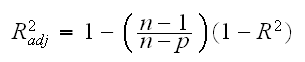
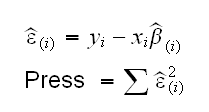
What is needed for selecting a "good" model is a measure that combines the quality of the fit and the "smallness" of a model. There are many methods known for this, here are some:
• adjusted R2:
• PRESS (predicted residual sum of squares) is a measure based on cross-validation:
• Mallow's Cp
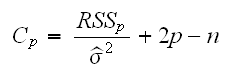
All of these methods work fine in most cases. We will mostly use Mallow's Cp.
How do we use these methods? As long as there are not to many predictors we can simply run all possible regression models and pick one that has the best (lowest) Cp. This is called "best subset" regression. Of course if there are p predictors in the full model there are 2p possible models, so this can take a long time quite easily. In the highway dataset there are 13 predictors, so there are 213=8192 different models. In
highway.fun(5)
we use the library "leaps" which does the computations, and we print out the 5 models with the lowest Cp's.
It is important to remember that Cp is a statistic, that is a random quantity with an error. So it is not clear whether the model using (len, slim, sigs, cpt, pa) with Cp=-0.38 is really better than the model using (len, slim, acpt) with Cp=0.24.
Clearly a modern PC can handle this size problem, but what do we do if it does take to long to run the full best subset regression? In that case we might try and use some knowledge of the subject matter, which is a very good idea at any rate. For example we notice that variables fai, pa amd ma are dummy variables that together describe the type of road used. So we should only look at models that either have all three variables in them, or non at all. Another consideration is the variable len, the length of the highway. It is reasonable to assume that this variable should be included, no matter what the "statistics" say. With this we are now down to 210=1024 models. Unfortunately I don't know of any routine for R that would let us run the best subsets regression for this models.
Even using all our "subject-matter knowledge" there will still be problems with too many predictors to run a best subset regression. For those problems a variety of model-selection strategies have been invented. One of them is "backward selection":
• 1) Compute the model with all the predictors in it.
• 2) Compute all the models with one of the predictors left out.
• 3) If none of the models with one predictor left out is "better" than the full model, stop
• 4) If some are "better" find the predictor that gives the best improvement, drop this predictor from the full model and then go back to 2.
"better" here can be any of the measures described above. Because we are now comparing "nested" models, that is the predictors in one model are a subset of the predictors in the other model, we can also use the F-test.
In R there are some special funtions to carry out this procedure. One is drop1 which computes all the models with one predictor left out and the other is update which recomputes the fit with a specified predictor left out. In
highway.fun(6)
we carry out the first step. We find that shld is the least significant variable (F=0.0076) and so we remove it from the model.
In
highway(7)
we continue on. We drop variables as follows:
2) lane, F=0.0089
3) adt, F=0.0051
4) fai, F=0.1368.
Because of the discussion above we now also drop pa and ma.
5) lwid, F=0.3471
6) itg, F=0.4025
7) trks, F=1.1329
8) sigs, F=2.0185
At this point the remaining variables len, slim and acpt all have large F-values (or small p-values) and so we stop.
Instead of "backward selection" we can also try "forward selection":
• 1) Compute all the models based on one predictor and choose the "best" of those model.
• 2) Compute all the models with one of the other predictors added on.
• 3) If none of the models with the new predictors is "better" than the old model, stop.
• 4) If some are "better" find the predictor that gives the best improvement, add this predictor to the old model and then go back to 2.
The function add1 helps with carrying out this method.
A third popular method is called "stepwise regression". Here we combine the forward and backward methods, that is in each step we check all the models with one predictor dropped or one predictor added to the current model and go to the best of those, if it is better than the current model.
highway(8)
runs the "step" command which carrys out this idea. It uses AIC (Akaike's information criterion) to choose between models. It comes up with a model based on len, slim, sigs, acpt and pa.
It is important to remember that none of these methods can be expected to work well all the time. A good policy is to use them all, and then compare the final models to see how they differ.