Example Consider that data in cats. It has been widely studied and analysed over the years, first by Sir R.A. Fisher.
Let's have a first look at the data
attach(cats)
summary(cats)
Fisher's interest in this dataset was to study the variation of heart weight with body weight and to discover if this differs by sex.
Ignoring sex for the moment we can draw the scatterplot
plot(Bwt,Hwt)
and we see that the heart weight and the body weight are positively correlated. In fact
cor(Bwt,Hwt)
is 0.804. Of course we could do Pearson's test for H0: ρ=0:
cor.test(Bwt,Hwt)
which has a p-value of 0.000 and therefore shows that the correlation is statistically significantly different from 0, although that test is clearly not necessary here.
Now let's include Sex:
qplot(Bwt,Hwt,color=Sex)
another nice way to do this is by using plotting symbols that identify the gender directly:
plot(Bwt,Hwt,pch=ifelse(Sex=="F","F","M"),col=ifelse(Sex=="F","red","blue"))
If this is to messy we could separate the two graphs
xyplot(Hwt~Bwt|Sex)
What are the correlations?
cor(Bwt[Sex=="F"],Hwt[Sex=="F"])
cor(Bwt[Sex=="M"],Hwt[Sex=="M"])
The correlations for both females and males are smaller than for the combined data. Any idea why that might be?
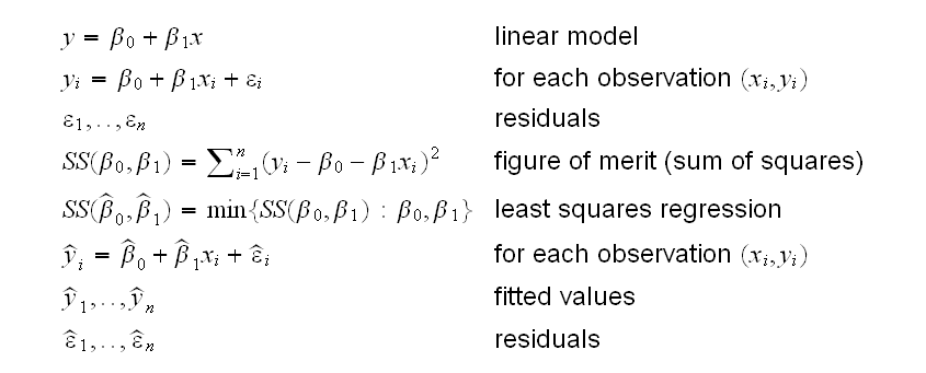
From the graphs it appears that the relationship between Body weight and Heart weight is linear, so we can try to fit a linear model. One way is to use the method of least squares regression:
Let's again ignore sex for the moment:
fit=lm(Hwt~Bwt)
sumary(fit)
"fit" is a special, rather complicated data structure in R. Such objects often have methods already implemented for them. For example an object of class "lm" has the following methods:
• summary() prints useful information.
• coef() gives the coefficients of the model (β0, β1,..).
• resid() finds the residuals
• fitted() finds the fitted values
• deviance() finds the residual sum of squares
• anova() finds the sequential analysis of variance table
• predict() predicts the mean response for new observations
• plot() draws a series of diagnostic plots
Note that in this problem it might make good sense to fit a no-intercept model of the form y=β1x (why?) This can be done using the command
fit=lm(Hwt~Bwt-1)
Is this a good model?
plot(fit)
draws a number of graphs. The first is the residual vs fits plot which shows this model to be quite ok.
Now let's include sex. How about fitting a linear model for both sexes? One way to do this is to just use the command
fitF=lm(Hwt~Bwt-1,subset= Sex=="F")
fitM=lm(Hwt~Bwt-1,subset= Sex=="M")
Another is to use the variable "Sex" as an additional variable, that is fitting the model Hwt~Bwt+Sex:
fit=lm(Hwt~Bwt+Sex-1)
But what does this do? After all Sex is a categorical variable with values F and M, and least squares regression needs numbers. Obviously R codes Sex as numbers somehow. Let's try and find out how:
summary(fit)
shows the result of the fit. Now
predict(fit,newdata=data.frame(Bwt=2,Sex="F"))
predict(fit,newdata=data.frame(Bwt=2,Sex="M"))
predict(fit,newdata=data.frame(Bwt=4,Sex="F"))
predict(fit,newdata=data.frame(Bwt=4,Sex="M"))
(15.88812-7.736585)/2
(15.80603-7.654488)/2
are the slopes of the lines for the females and the males. They are the same, so we have parallel lines, and they are the "Estimate" of Bwt in summary(fit). The intercepts are
7.736585-2*4.075768
7.654488-2*4.075768
which are the coefficients of SexF and SexM in summary(fit). So this yields models Hwt=4.08Bwt-0.41I"{F"}-0.50I{"M"} or Hwt=3.91Bwt-0.41 for females and Hwt=3.91Bwt-0.50 for males. Notice that nopw despite the "-1" we again have intercepts. This is unavoidable because we fit parallel lines.
Exactly how does R do the coding?
x=ifelse(Sex=="F",0,1)
fit1=lm(Hwt~Bwt+x)
summary(fit1)
What does this fit look like?
plot(Bwt,Hwt,pch=ifelse(Sex=="F",3,4),col=ifelse(Sex=="F","red","blue"))
abline(coef(fit)[2],coef(fit)[1],col="red")
abline(coef(fit)[3],coef(fit)[1],col="blue")
legend(2,20,c("Female","Male"),lty=c(1,1),col=c("red","blue"))
So this fits two parallel lines. From the scatterplot it is already doubtful that this is a good model. Let's check the residual vs. fits plot, with a non-parametric (using a method called lowess, which is similar to loess) fit added:
xyplot(resid(fit)~fitted(fit)|Sex, panel = function(...) {panel.xyplot(...,type=c("p","smooth"))})
shows that the model is bad, certainly for the females.
In the command above panel.xyplot() determines what is drawn in the graph The choices are type="p", "l", "h", "b", "o", "s", "S", "r", "a", "g", "smooth", and (sometimes) we can combine them. Try some out!
xyplot(Hwt~Bwt|Sex, panel = function(...) {panel.xyplot(...,type=c("r","p","smooth"))})
What we need to do is fit separate lines as we did above, but we really want to do this in just one model, so we need to include an interaction term:
fit=lm(Hwt~Bwt+Sex+Sex*Bwt)
or
fit=lm(Hwt~Sex*Bwt)
summary(fit)
Again, what does that look like?
plot(Bwt,Hwt,pch=ifelse(Sex=="F",3,4),col=ifelse(Sex=="F","red","blue"))
abline(coef(fit)[1],coef(fit)[3],col="red")
abline(coef(fit)[1]+coef(fit)[2],coef(fit)[3]+coef(fit)[4],col="blue")
legend(2,20,c("Female","Male"),lty=c(1,1),col=c("red","blue"))
What are these lines if we write them down for males and females separatey?
Female:
y=β0+β1I("M")+β2Bwt+β3Bwt×I("M")=
y=β0+β10+β2Bwt+β3Bwt×0=
y=β0+β2Bwt=
y=2.98+2.63Bwt
Male:
y=β0+β1I("M")+β2Bwt+β3Bwt×I("M")=
y=β0+β1×1+β2Bwt+β3Bwt×1=
y=(β0+β[1])+(β2+β3)Bwt=
y=(2.98-4.17)+(2.63+1.68)Bwt
y=-1.19+4.31Bwt
The same model can be fitted explicitly, and withoud the need for any arithmetic, using the command
fit=lm(Hwt~Sex/Bwt-1)
summary(fit)
is this a good model? Again we can draw the residual vs. fits plot, with a non-parametric fit:
xyplot(resid(fit)~fitted(fit)|Sex, panel = function(...) {panel.xyplot(...,type=c("p","smooth"))})
We now have two ways to use the factor Sex in our linear regression: as parallel lines and as independent lines. There is a third:
z=ifelse(Sex=="F",0,Bwt)
fit=lm(Hwt~Bwt+z)
summary(fit)
which fits:
Female:
y=β0+β1Bwt+β2Bwt×I("M")=
y=β0+β1Bwt+β2Bwt×0=
y=β0+β1Bwt=
y=-0.34+4.028Bwt
Male:
y=β0+β1Bwt+β2Bwt×I("M")=
y=β0+β1Bwt+β2Bwt×1=
y=β0+(β1+β2)Bwt=
y=-0.34+4.03Bwt
or an Equal Intercept Model
Note that to fit this model we made a new variable z, just fitting
fit=lm(Hwt~Bwt+Sex*Bwt)
summary(fit)
is a different model. This is because in R a*b is interpreted as a+b+a:b. One way to fit this model without the z is to expicitely remove Sex from the model:
fit=lm(Hwt~Sex*Bwt-Sex)
summary(fit)
Using the method of least squares to find the equation is always "legal" but not always a good idea.
lm.exa(1)
shows some cases where the least squares regression line is clearly not a good model for the data.
All the other parts of the output of summary() have the additional condition εi~N(0,σ). Notice that this has two parts:
1) The residuals have a normal distribution
2) The standard deviations are all the same (homoscatasticity)
We can check these as follows:
1) Draw the normal probability plot of the residuals (It is already part of the plot() routine)
2) Check the residuals vs. fits plot again and look for a change in variance from left to right.
lm.exa(2)
shows an example with non-constant variance. Notice that this problem is almost "invisible" in the scatterplot of the data.
For the cats data the normal assumption appears to be fine but there is a slight hint of unequal variance.
One way to try and deal with the problem of unequal variance is to use a transformation. In our case we really are interested in testing Hwt~Bwt. If this is so then Hwt/Bwt should be a constant. So we will now consider the model
log(Hwt/Bwt)=β0+β1log(Bwt)+ε
plot(log(Hwt/Bwt),log(Bwt))
shows no indication of a relationship.
fit= lm(log(Hwt/Bwt)~Sex/log(Bwt))
summary(fit)
shows an F-statistic of 1.46 on 3 and 140 df with a p-value of 0.229, which indicates that the total contribution of the model beyond the constant is negligible, suggesting that in both sexes heart weight is proportional to body weight and that the constant of proportionality is the same for both sexes.
Using the F-statistic for this question is not the same as looking at the individual t-tests. Why not?
plot(fit)
shows that the log transformation was succesful in removing the heteroscatasticity.