Generalized Linear Models

Generalized linear models (GLMs) extend linear models to include both non-normal response distributions and transformations to linearity. The most important reference is McCullagh and Nelder (1989)

An Introductory Example

Example We begin with a very famous dataset from the Challenger shuttle disaster. In

shuttle.fun(1)

we draw the scatterplot and observe a tendency for failures at lower temperatures. In

shuttle.fun(2)

we redraw the graph and use as the response variable an indicator variable of whether or not a failure has occured. Note that in this graph several points repeat (for example (70,1)) and we use some jittering on the x-axis to make them all visible.

What we would like to do is develop a model for predicting "failure" from "temperature". But here the response variable "failure" is a discrete variable, actually it has a Bernoulli distribution with "success" (!) probability p. So rather than trying to predict "failure" we will try to predict p. This is done via logistic regression:

We have reponses Y₁, .., Y_n iid Bernoulli(p). So E[Y_i] = p. We assume that p is related to the predictor x via the equation

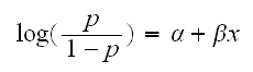
the left-hand side is the log of the odds of success for Y and is called the logit link function. It is a natural model in this case because for the Bernoulli distribution we can write the probability mass function as follows:

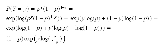
and so the term log(p/1-p) is the natural parameter of this exponential family. When the natural parameter is used in this way it is called the canonical link.

Notice that solving the model above for p we find

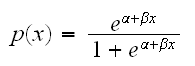
which does not allow for the possibility of p=0 or p=1. If we have a problem were these cases are releveant we would need to use a different link function.

Notice that as in simple linear regression if β=0 we have the case of no relationship between x and y. It can also be shown that β is the change in the log-odds of success corresponding to a one-unit increase in x.

How do fit such a model, that is find α and β? For linear regression we used the method of least squares, which was possible because we could directly compare x and y. This is not the case here because p and x have different forms, which is why we needed a link function. Instead we will use maximum likelihood for the estimation. The log-likelihood is given by

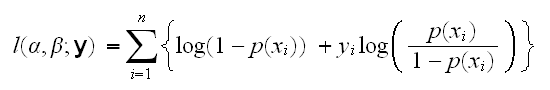
and we can then find the mle's by differentiation. In R this is done using the command glm with family=binomial, which we run in

shuttle.fun(3)

In

shuttle.fun(4)

we draw the fitted line plot where we see that at the expected launch temperature of 32°F the failure probability is 1.

Can we add a confidence band to the graph? As with other predict commands the one for glm will calculate has an argument se.fit. Using that and finding Normal theory intervals we get

shuttle.fun(5)

but that looks very strange! In fact the bounds go below 0 and above 1, which of course makes no sense.

The problem is that we calculated the errors in the scale of the probabilities. Now adding ±z_α/2s is likely to "push" the limits above 1 and below 0.

What we need to do is calculate the errors in the scale of the linear model, that is for log(p/(1-p)), then transform everything to the scale of the probabilities. This is done by using the type="link" argument instead of type="response", see

shuttle.fun(6)

Is this actually ok? That is, are this proper confidence intervals? The answer is yes, because if f is a monotone function we have

1-α = P(L(X)<θ<U(X)) = P(f(L(X))<f(θ)<f(U(X)))  

One other comment: Obviously predicting the o-ring failure probability at a temperature of 32°F is an extrapolation, with the usual dangers. But even if the true probability had been only 50%, the decision would certainly have been to postpone the lauch.

The General Theory

A generalized linear model has the following components:

1) There is a response, y, observed independently at fixed values of stimulus variables x₁, .., x_p
2) The stimulus variables may only influence the distribution of y through a single linear function called the linear predictor
h=β₁x₁+ ..+ β_px_p

3) The distribution of y has a density of the form
f(y_i|θ_i,j)=exp[A_i{y_iθ_i-γ(θ_i)}/j+t(y_i,j/A_i)]
where j is a scale parameter (often known), A_i is a known prior weight and parameter θ_i controls the distribution of y_i.
4) The mean μ is a smooth invertible function of the linear predictor:
μ=m(h), h=m^-1(μ)=l(μ)

It can be shown that θ=(γ')^-1(μ)

If j is known the distribution of y is a one-parameter exponential family.

There are many standard problems that fit into this general framework:

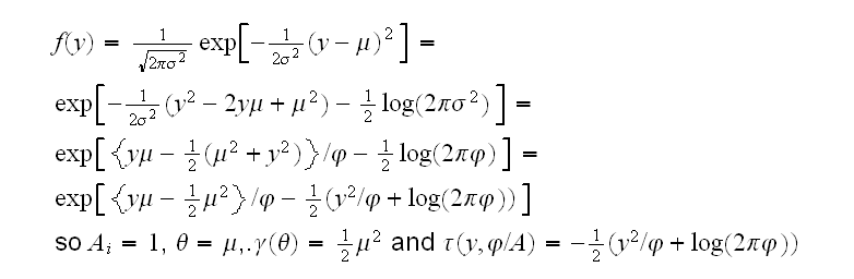
Gaussian For the normal distribution j=σ² and we have

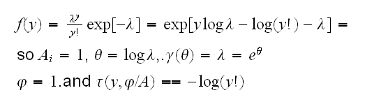
Poisson Now

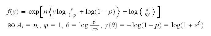
Binomial for the binomial distribution with a fixed (known) number of trials n and success parameter p we take the response to be y=s/n where s is the number of successes. Then

The functions for GLMs included in R are gaussian, binomial, poisson, inverse.gaussian and gamma.

Each response distribution allows a variety of link functions to connect the mean with the linear predictor Those automatically available are:

Link	binomial	gamma	gaussian	inv.gaussian	poisson
logit	D	•
probit	•
cloglog	•
identity		•	D		•
inverse		D
log		•			D
1/μ2				D
√					•

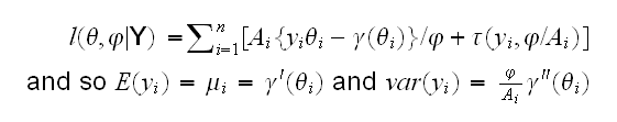
Say we have n observations from a GLM. Then the log-likelihood is given by

Poisson Data

Example As an example consider the Experiment in Soldering.
As a first look we draw the histogram of the response skips, in

solder.fun(1)

This has the skewed to the right appearance typical for Poisson data. Another look at the data is in

solder.fun(2)

where we plot the mean response for for each level of the predictors, an alternative to looking at the boxplots which we do in

solder.fun(3)

The two factors with the greatest effect on skips are Opening and Mask.

solder.fun(4)

fits the GLM on the five predictors, and check the ANOVA table. Clearly all five factors are highly significant.

Do we need to worry about interactions?

solder.fun(5)

refits the model and include all the second order terms. Indeed almost all of them are significant.

signal.fun(6)

checks the assumptions.

It often helps to understand what a method does to do a simple little simulation. In

glm.sim(1)

we generate data as follows: we let x be 100 equal spaced values from 0 to 1 and generate 100 values λ for the rates of a Poisson random variable using log(λ) = -1 + 4×x + N(0,0.15). Then we generate 100 observations y~Pois(λ). We also print out the coefficients of the glm fit, which match the true values quite well. Because Ey=λ for the Poisson distribution we can even include the fitted line in the plot.

How do we find confidence intervals? Of course there is a predict method, and it yields the standard error using se=T. Say we want to find a 95% CI for λ if x=0.5. The true answer of course is λ=exp(-1+4*0.5)=e¹=2.71828. We find the limits in

glm.sim(2)

Are this good confidence intervals? In

glm.sim(3)

we do a small coverage study and find the limits to work quite well.

Birth Weights

Example As another example consider the Birth Weights dataset. Although the actual birth weights are available, we will try to predict whether the birth weight will be low (less than 2.5kg).

Notice that there are only a few observations with 'ptl' greater than 1. Also, it is probably unreasonable to expect a linear model in 'ptl'. For those reasons we turn 'ptl' into a dummy variable indicating past history. Similarly 'ftv' is reduced to three levels.

In

birth.fun(2)

we fit the glm with family="binomial", and also use the step function for stepwise selection. Then we see how many of the cases in the dataset are correctly predicted.