For a linear regression we have a dependent variable Y and a set of predictors X1, .., Xn and a model of the form
Y = α + ∑ βjXj + ε
Generalized additive models extend this in two ways: first we replace the linear terms βjXj by non-linear functions, to get
Y = α + ∑ fj(Xj) + ε
Second we can take the same step as before in going from linear models to generalized linear models to fit problems where Y is a categorical variable.
Some special cases we have already discussed:
• The functions fj are polynomials
• We have just one predictor, see the discussion on local regression models.
We can also "mix" linear and generalized additive models. Consider
Y = α + β1X1 + β2X2 + β3X22 + β4f(X3) + ε
here we have a model linear in X1, quadratic in X2 and additive in X3. Such a model is called "semiparametric"
Example Let's have a look at the Rocks dataset. In
rock.fun(1)
we look at the boxplots, and we see that the response perm is somewhat skewed to the right, so we will use a log transform on perm. In
rock.fun(2)
we have a look at the scatterplots of log(perm) vs. the predictors, and we see some slight relationships, with peri being the strongest. Let's first continuoue as before and fit a linear model, done in
rock.fun(3)
In fact the linear model does not appear that bad. Next let's fit the generalized additive model. This is done in
rocks.fun(4)
using the function gam. Notice the terms s() which means we are using splines.
Is this model better than the simple linear one? We can compare the two using ANOVA, done in
rock.fun(5)
It appears the more complicated model is not actually better than the old one.
What is this new model? In
rock.fun(6)
we have a look at the fitted line plots. Using se=T adds confidence intervals, but be careful! These are pointwise confidence intervals, not simultaneous confidence bands.
It appears that at least area and peri have a linear relationship with log(perm), so maybe we should fit a linear model in these variables. This is done in
rock.fun(7)
where we again compare it to the linear model and in
rock.fun(8)
where we look at the fitted line plots. Again it seems the linear model is adequate.
Example Next we have a look at the dataset Kyphosis. In
kyphosis.fun(1)
we look at the boxplots and see a strong relationship between Kyphosis and Start as well as Number. We also print out some summary statistics.
Here the response variable Kyphosis is binary, so we will use logistic regression to model the data. This is done in
kyphosis.fun(2)
Is the relationship between the predictors and Kyphosis really linear? Again we check this by fitting instead a generalized additive model, in
yphosis.fun(3)
It does appear that some of the relationships are not linear.
How can we do a little bit of model selection, that is simplifying the model by possibly leaving out some predictors? Let's use a "forward selection" method. In
kyphosis.fun(4)
we fit a model using just Start and then a model with Start and Number. Using anova we compare the two and see that Number does not add anything to the model. Doing the same thing with Age shows Age to be useful, though.
Can we simplify the model in other ways? One problem with non-parametric or local regression models is that they are very difficult to interpret, so replacing these fits with some explicit functions would be useful. In kyphosis.fun(5) we look at the splines used for the fits on Start and Age. From this it seems a model quadratic in Age might work. For Start we see that its spline appears piecewise linear, flat up to about 12 and then with a negative slope. This also makes sense from the background of the data, because values of Start up to 12 correspond to the thoracic region of the spine and values greater than 12 belong to the lumbar region. We will therefore try and fit a model of the form
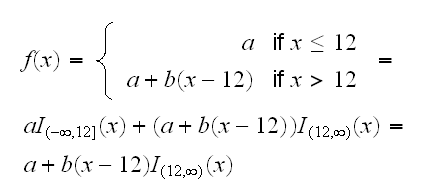
Notice that this model fits a continuous function. In R we can do this by including a term I((Start-12)*(Start>12)), which is done in kyphosis.fun(6). The 'I' is needed so R does not interpret the '*' as meaning interaction. Comparing this with the gam model we see that this model is as good as the generalized additive one.
What does this new model look like? In kyphosis.fun(7) we see what the functions look like, and in kyphosis.fun(8) we have a look at the predicted probabilities depending on Age and Start.
Example Next we have a look at the Spam dataset. In
spam.fun(1,T)
we fit a generalized additive model with the logit link to the data. WARNING: it takes about 10 min to run. The result is in spam.fit[[1]], which is shown in
spam.fun(1)
There is a small "technical" problem here : gam(spam~.) fits a model linear in the predictors and gam(spam~s(.)) does not work. There is probably an elegant way to do this, but I don't know it, so here is a "workaround" saving the time to type it all in: use paste("s(",names(spam),")+",collapse="") and the copy-paste it into the function.
spam.fun(2)
refits, using only the "significant" variables from the full model. We already know that judging the importance of a variable based on the individual tests is usually not a good idea, but given how long even a single run of gam takes anything else probably requires a super-computer and a lot of time.
spam.fun(3)
we look at the coefficients and the p-values of the resulting model. Note that a positive coefficient makes it more likely that an email is spam, and a negative one makes it less likely.
How good a model is this? Well, we use it to predict whether or not an email is spam, so how well does it do the job? We do this in
spam.fun(4)
and see that it gets it right about 95% of the time. This though is probably to optimistic, because we are testing the performance on the same dataset we used for fitting the model, which usually results ina bias. Instead we can do the following:
• randomly devide the data in a training set (size=3000) and an evaluation set
• fit the model using the data in the training set
• evaluate the performance using the data in the evaluation set, which is independent from the training set.
This is done in
spam.fun(5)
and
spam.fun(6)
with the results shown in
spam.fun(7)