Example Let's consider the lengths of the eruptions of the Old Faithful Guyser. This is data from a continuous random variable and therefore has a density f. We would like to estimate that f, that is f(x) for all x.
As a first try we should have a look at the histogram of the data:
faithful1.fun(1)
does four of them, for different numbers of bins. It appears f is bimodal, with one peak at about 1.75 and a second one at about 4.5
The main problems with the histogram are that it is discontinuous, with jumps at the bin edges, and its dependence on the left edge. As a first try to resolve this problem we could decide on a likely shape of the density, and then use some fitting. In the case of the eruptions we have a bimodal density, so maybe a mixture of two normal densities might work. From the histogram it appears we have a N(1.75,0.5) and a N(4.5,0.5). Using the EM algorithm we get the maximum-likelihood fit
faithful.em()
Not at all bad. The main problem of course is the justification of the normal mixture, why not two Student t's for example? Or Gammas, after all the eruption times have to be positive. And so on.
A completely different apprach is via non-parametric density estimation. As the name suggests this does not make any assumptions about the shape of the density. There are now a number of methods known, with the most common one being
Kernel Density Estimation
Let's go back to the histogram for a second. There are two "obvious" ways to draw a histogram, either showing the counts or the percentages. We want the histogram to be a density, though, so it should "integrate" out to 1. How do we find the height of the histogram bars? Let fk be the number of observations in bin [bk,bk+1) then
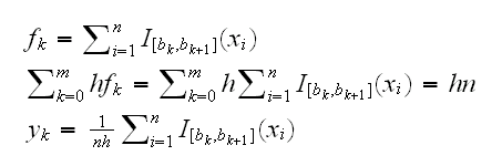
the idea is then to replace the indicator function with a smooth function, centered at the midpoint of the interval and symmetric. There are a number of such kernels:
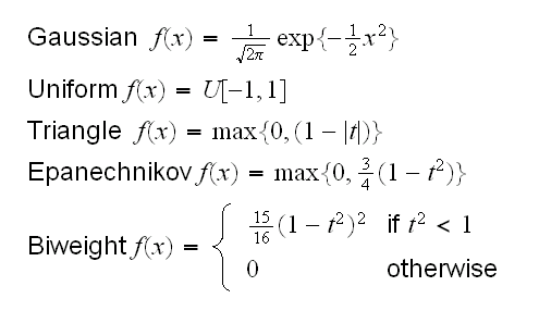
Notice that each of these kernels is itself a density. This is not strictly necessary but makes the math easier.
In general the kernel is not of great importance, all of these work fine. Epanechnikov seems like a good choice because of the ease of calculation.
faithful1.fun(3)
draws the histograms together with these density estimates.
The most important question is of course the choice of the bandwith h.
faithful1.fun(4)
draws several of them, but is there an optimal choice? As always when looking for an "optimal" choice we need first to decide what "better" means, that is we need a criteria to judge how well an estimate works. And again as (almost) always is Statistics, there are different criteria one can use. In parametric estimation one often considers the variance of the estimator. Here this will not work because it can be shown that non-parametric density estimators are always biased (a result due to Rosenblatt 1956), and this bias needs to be included in our criterion. If we were interested in the estimation of f at the point x we could consider
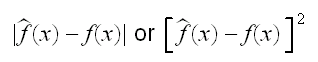
but of course we want an overall criterion for all x simultaneously. Again there are several choices:
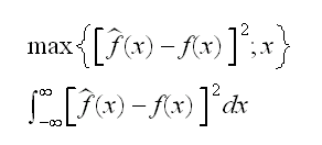
But the density estimate also depends on the data, so finally we come to the mean integrated squared error:
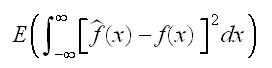
It can be shown (using Fubini's theorem from real analysis) that MISE=IMSE.
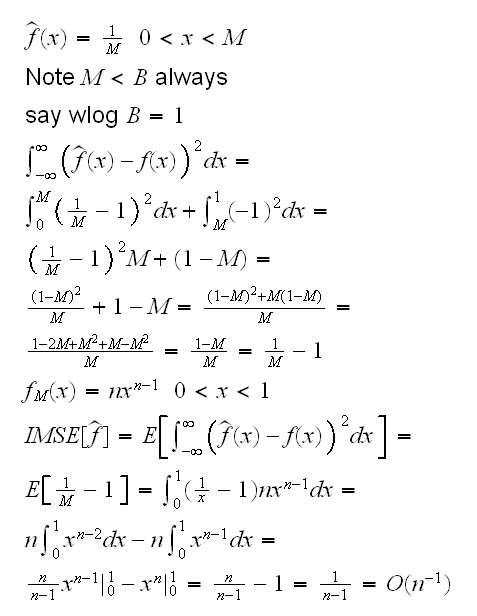
Let's study this criterion in a simpler context, that of parametric estimation:
Example say f is the density of a U[0,B], that is f(x)=1/B if 0<x<B. Then the mle of B is M=X(n), the nth order statistic (or maximum) so
let's get back to non-parametric density estimation:
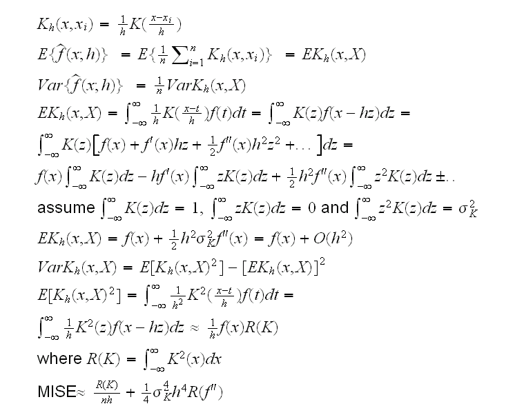
Now say we want to minimize MISE, then
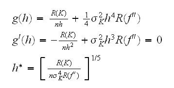
Sounds great except we are trying to find f, so we don't know f'' either. Nevertheless, some progress has been made. In
faithful1.fun(3)
we aleady drew the densities using different Kernels but the same h, and it is clear that an h that leads to a smooth curve for one kernel might be quite ragged for another. Say we have used Kernel 1 with bandwith h1, and we decide to switch to Kernel 2. What bandwidth h2 will result in the same estimate? The above suggests the following:
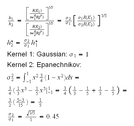
In
faithful1.fun(5,h=0.4)
we draw the curves with these equivalent bandwidths.
Optimal Bandwidths
To begin with, if we assume a parametric form for the density we can find an h that is optimal for that shape. For example if we know that the data has a normal distribution with standard deviation σ and using a Gaussian kernel we find h*=1.06σn-0.2 to be minimizing the MISE. In
faithful1.fun(6)
we generate 1000 observations from N(0,1) and add the respective estimate.
This may not appear to be much, after all if we know the shape we don't need non-parametric density estimation, but at least it gives us a starting point.
Another approach is to find an upper bound on h, the socalled oversmoothed bandwidth hOS. It can be shown that
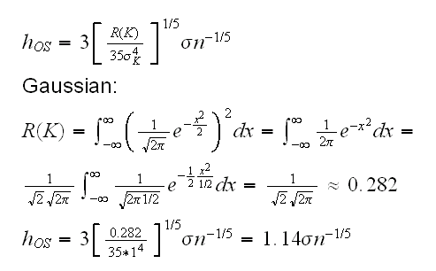
slightly large than the normal reference rule.
Finally we can try to find an optimal choice of h based on cross-validation. If we use the Gaussian kernel, then the unbiased cross-validation score UCV(h) can be shown to be
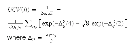
The function ucv.fun calculates this, and
faithful1.fun(7)
draws h vs UCV(h) for x a sample of size 100 from N(0,1)
faithful1.fun(8)
does the same thing for the eruptions
Obviously this is very slow even for small datasets. There are much faster implementations of this available, as part of the MASS, see
faithful1.fun(9)