Notice that we are not saying there is no difference between Toxins 1 and 3, only that based on our sample sizes and 95% confidence intervals we can not be sure that they are different.
ANOVA can be studied as a special case of a linear model where the response variable is continuous but all the predictors (now called factors) are discrete.
Example we start with the dataset on the relative effects of toxins on the liver of trout.
trout.fun(1)
finds the table of summary statistics (sample sizes, means and standard deviations) and also draw the boxplot. From this it appears clear that not all 4 groups have the same means.
In order to verify this we can run the ANOVA. In R this is done with the aov command, which we use in trout.fun(2). The overall hypothesis of equal means has an F value of 26.093 with a p-value of 0.00, and so we clearly reject this hypothesis. The diagnostic plots show no problems with this analysis.
Of course we usually want to go a little further, and study the individual differences, for example, is "Control" stat. sign. different from "Toxin 3"? This goes under the heading of "multiple comparisons". There are numerous methods known for carrying out a multiple comparison study, unfortunately non of them is part of the standard distribution of R. Again, though, at StatLib we find multcomp, a package to carry out a multiple comparison study. (It also needs the library mvtnorm)
We run the routine glht
trout.fun(3)
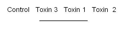
using Tukey's multiple compariosn method. We find that the only difference that is not found to be stat. sign different from 0 is between Toxins 1 and 3. A nice way to summarize the result of a multiple comparison study is as follows: sort the factors by their means, and underline together those that are not declared to be different:
Notice that we are not saying there is no difference between Toxins 1 and 3, only that based on our sample sizes and 95% confidence intervals we can not be sure that they are different.
The obvious way to look at this type of problem is to consider the data to come from different groups and to ask whether the group means are the same. So how does this fit into the framework of linear models? Instead of phrasing the problem as one with data from different groups we can again phrase it has having a predictor ("treatment") and a response ("amount") and asking whether there is a relationship between the two.
In the context of ANOVA the preditors are usually called factors, for historical reasons.
We can then consider models of the form
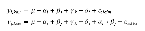
Here μ is the overall mean response, that is our best guess for the response if we do not know anything else. αi is the change from the overall mean reponse due to the fact that the observation yijklm comes from the ith group of the 1st factor, etc. Testing whether the first factor is significant then means testing H0: α1=α2=..=αp=0.
Terms like αi•βj model the interactions of the factors.
Example as another example let's consider the Absences from School dataset. There are 146 children in our dataset.
table(Lrn, Age, Sex, Eth)
shows the design to be highly unbalanced, in fact a number of factor-level combinations do not appear at all.
A good first look at the data is given by the boxplots of response vs. factors:
quine.fun(1)
This shows that the response is skewed to the right, and not normal as is required for ANOVA. Often this can be "fixed" by a transformation. Now the only continuous variable is the response, so that's the only one we can transform. Rather than simply guessing we might use the Box-Cox transforms.
quine.fun(2)
draws the Box-Cox transforms. It shows that values between 0.1 and 0.35 are acceptable.
It is usually desired, though, to find a "nice" transform, such as 1/y, √y, log(y) etc. Unfortunately none of the values allowed by the Box-Cox transform yields such a nice transform. Instead we can try and use a "displaced" log transform with t(y,α)=log(y+α). Again an optimal value of α can be found analogously to the Box-Cox method. It yields an optimal value of α=2.5.
In
quine.fun(3)
we run three examples, from the simple model without interactions to the full model with all possible (linear) terms.
In the full model the following terms are stat. sign. (at the 5% level): Eth, Eth•Age, Eth•Sex•Lrn. Of course we would like to find a model with the fewest possible factors (a parsimonious model), and it would be tempting to now choose those three. Generally this will not work, we need a different method for model selection. As before we can use backward selection.
A term such as A•B is said to be marginal to any higher order term that includes it, such as A•B•C. If both occur in a model then discarding marginal terms does not affect the statistical meaning of the model, only the way it is parametrized. So when removing terms from a factorial model we can concentrate on currently non-marginal terms.
In the full model the only non-marginal term is Eth•Sex•Age•Lrn, which is non-significant. In
quine.fun(4)
we drop the four-way interaction term from the model and show the resulting model. In
quine.fun(5)
we use the drop1 command to examine the effects of dropping the next highest-order non-marginal terms from the model. Of the 4 Eth•Sex•Age has the smallest F-value (with a p-value greater than 0.05), so it is dropped next
quine.fun(6)
and we continoue in this manner.
quine.fun(7)
to
quine.fun(10)
Eventually we arrive at a model which has no more terms that can be dropped.
quine.fun(11)
shows the information for this model. Note that is contains many terms which had a p-value greater than 0.05 in the full model.
Our final model is the best of those examined, but it need not actually be a correct model at all! Again we need to check the assumptions, and again we use the diagnostic plots as before
quine.fun(12)
We can again use the "stepwise" procedure to do the model-selection. It is run in
quine.fun(13)
Note that its final model includes three more terms than the one above.
Our final model (from the backward elimination method) is
log(Days+2.5)=Eth+Sex+Age+Lrn+Eth•Sex+Sex•Age+Eth•Lrn+Sex•Lrn+Eth•Sex•Lrn
Probably the most important question in an ANOVA problem is this: what does this mean? how can we interpret this model? what does it tell us about the underlying process? Unfortunately this is also the hardest question, at least if there are interaction terms.
Example Let's look a the Poison dataset. In
poison.fun(1)
we look at the summary of the dataframe "poison" and we see that we have 12 observations for each treatment and 16 observations for each poison, so we have a balanced design. We also look at a table of factor-level combinations, and we see that each combination appears 4 times, so we have a design with replication.
We have 2 factors in this dataset, poison and treatment. This type of problem comes in two forms, called either a randomized block design or a factorial experiment. Ours is a factorial experiment. So to summarize, we are looking at a balanced two-way factorial design with replicates.
poison.fun(2, Mean=T)
finds the mean and the standard deviation of surv.time for each factor-level combination, and also plot these means in a design plot. Here this plot is perfectly nice, at other times (if there are outliers, for example) we might better use the median and the interquartile range, see
poison.fun(2, Mean=F)
poison.fun(3)
draws the boxplots, where we see sizable differences between the levels of both factors.
Another useful graph is the interaction plot, done in
poison.fun(4)
or
poison.fun(5)
where we see a slight hint of interaction.
poison.fun(6)
runs the ANOVA for the model with interaction, checks the assumptions and looks at the summary. The assumptions look fine, and in the summary we see that both factors are highly significant whereas the interaction term is not.
poison.fun(7)
reruns the ANOVA but only for the first 12 rows of the dataframe. As we see now the ANOVA table only goes to the Mean Sq but no longer includes the hypotheses tests. This is because now we have no replications, and then the test for the interaction term is no longer possible. We can at least do the tests for the factors by fitting an additive model, but this might be wrong if there is indeed interaction present.
How about multiple comparisons? Because we have seen that there is no interaction we can run the multiple comparisons separately for treatment
poison.fun(8)
and poisons
poison.fun(9)
We find stat. sign differences between treatments A and B as well as B and C, and between poisons I and III as well as II and III.
If there is interaction, then running individuel multiple comparisons will generally not work. In that case we can try the following: instead of treating this a two-way factorial design we look at it as a one-way design with a factor TreatmentPoison with 12 levels "AI", "AII", .., "CIII", and run the multiple comparison on that. This is done in
poison.fun(10)
Note, though, that here we have 12 factor-level combinations, so there are 12 choose 2 or 66 pairs, which means the routine takes some time to run and the result is not very informative.
When analyzing this type of data it is very important to distinguish between balanced and unbalanced designs. The usual ANOVA formulas all assume that the design is balanced, and don't always work if it is not. As an illustration consider the artificial dataset generated in ubd.fun (taken from Freund and Wilson, p.349). Here we have an unbalanced two-way factorial design with factors A (levels 1 and 2) and B (levels 1, 2 and 3). In
ubd.fun(1)
we find the means for A (5.86 and 4.14) which are quite different. Running the ANOVA we see that factor A has a p-value of 0.0416, so it is significant at the 5% level. But in
ubd.fun(2)
we find the means for each factor-level combination, and we see that the means of A for the same level of B are identical! The apparent difference in means of A are in fact due to factor B.
Another difficulty is this: in
ubd.fun(3)
we do the ANOVAs response~A*B and response~B*A, and they are not the same! This again is a consequence of an unbalanced design. In
ubd.fun(4)
we rerun the ANOVA for the poison dataset, and we see that there the order in which the factors are used does not matter.
How can we correctly analyze this dataset? We do this by turning it into a regression problem using dummy variables. In
ubd.fun(5)
we construct variables A2 (an indicator variable for level 2 of A), B2 (an indicator variable for level 2 of B) and B3 (an indicator variable for level 3 of B) and then run the usual regression on response (including all the interaction terms). The output shows that the tests for B2:B3 and for A2:B2:B3 are not possible, so we rerun the command with just the interactions that can be included. We see that A2 is highly non-significant, as we want.
It is not necessary to actually do the coding of the dummy variables "by hand", we can use the command glm (for general linear model) to do it for us, see
ubd.fun(6).
In general it is much easier to analyze balanced designs, which is a good reason to try and set up your experiment accordingly.
This was just a very short intro to ANOVA, the real fun starts when we want to analyze data from special designs such as magic squares, split plot designs etc. Take a course in the Design of Experiments!