Say we have a probability model and we want to find a quantity associated with the model. How can we do this? The first try should be to do it analytically:
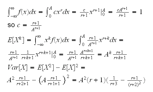
Example say we have a rv X with pdf f(x)=cxr, 0<x<A, A,r>0. We want to know Var[X]
Alternatevly we can try to use simulation: generate data from this distribution and find the corresponding sample quantity. To do that we need to generate data from this distribution. R has many probability distributions already built in, and generating data is done with a command like r"name"(, ...). For example if we want 1000 observations from a standard normal distribution : rnorm(1000). If we want a uniform on [1,2]: runif(1,1,2). Another useful command is sample: it takes a vector as its argument and samples from the elements of the vector. Say we want 1000 observations from (0,1,2): sample(0:2, size=1000,replace=T). Say we want the same but with probabilities (1/2,1/4,1/4): sample(0:2, size=1000,replace=T, prob=c(2,1,1)).
Example so how about our example? If you look at the density it has the form cxr, the same as the density of a Beta rv: cxα-1(1-x)β-1 with α=r+1 and β=1, except that a beta rv has values on [0,1], not [0,A]. But say Y~Beta(r+1,1) then
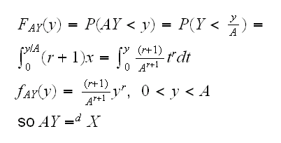
so we can generate data from f with A*rbeta(n,r+1,1)
This is very simple, but maybe its a good a idea to check anyway. For that let's generate 10000 variates, draw a histogram scaled to "intergate" to 1 and add the density curve, see
sim1(1,r=4)
What can we do if we need data from a distribution that is not already implemented in R? There are many methods known how to generate rv, we will discuss one of them called the accept-reject algorithm:
Assume we want to generate a r.v. X with density f. We have a way to generate a r.v. Y with density g. Let c be a constant such that f(x)/g(x)≤ c for all x. Then the accept-reject algorithm is as follows:
Step 1: generate Y from pdf g
Step 2: generate U~U[0,1]
Step 3: If U < f(Y)/(cg(Y)), set X = Y and stop. Otherwise go back to 1
We have the following theorem:
Theorem
The accept-reject algorithm generates a r.v. X with density f
In addition, the number of iterations of the algorithm needed until X is found is a geometric r.v. with mean c.
Example f(x)=(r+1)xr/Ar+1, 0<x<A. For the algorithm we need a rv Y we already know how to generate. For example here we can use Y~U[0,A]. Then
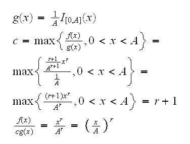
and the algorithm is
1) generate Y~U[0,A] with Y=runif(1,0,A)
2) gnenrate U~U[0,1] with U=runif(1)
3) if U<(Y/A)r set X=Y, otherwise return to 1
done in
sim1(2)
In order to see why this algorithm works check out
sim1(2,Show=T).
Simulation has some drawbacks: first we need to be able to generate the data, and then the result has some "simulation error", due to the fact we only generate finitely many variates. Finally, we can always only get a result for a specific value of the parameter, not a "formula" for all values. Still, if the calculation is to difficult it maybe our only answer:
Example say X,Y~Beta(2.5,0.9) and we want to know Var[(X/(X+Y)]. Doing this analytically is not impossible but would take even a good mathematician a couple of hours. Instead
x=rbeta(1000000,2.5,0.9)
y=rbeta(1000000,2.5,0.9)
var(x/(x+y))
shows that Var[(X/(X+Y)]=0.0148 and takes about 15 seconds to write and run.
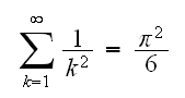
Example : say we want to generate r.v.'s X such that P(X=k)=6/(π2k2), k=1,2, ...
Recall
We need a r.v Y on {1,2,..} which we can generate. There are two "standard" discrete rv's which take infinitely many values, the Geometric and the Poisson. But there is a problem with those two:
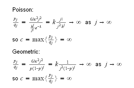
In both cases c is infinite because the probabilities P(Y=j) go to 0 much faster than P(X=j), so that pj/qj=P(X=k)/P(Y=k)→∞.
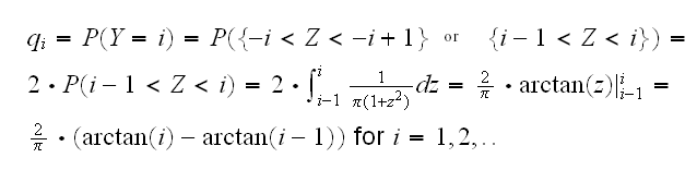
We do know, though, a continuous r.v. that goes to 0 very slowly, namely the Cauchy. Actually, its density f(x)=1/(π(1+x2)) already has the right "size" for our problem. We can do this, then by "discretizing" the Cauchy: Let Z~Cauchy and define Y=i(I[-i,-i+1](Z)+I[i-1,i](Z)) for i=1,2,.. So
if |Z|<1 → Y=1
if 1<|Z|<2 → Y=2
and so on. Then
Now we need max{pj/qj}. Doing this via calculus would be quite difficult because we would end up with a nonlinear equation which we would need to solve numerically. A different approach is to just plot j vs. pj/qj and see what it looks like. This is done in
sim2(100, findc=T)
We see that pj/qj appears to approach a limit a little below 1 as j goes to infinity, but it has a value of 1.216 at j=1, so we can reasonably guess that c=1.216 should work for us. (Of course we can verify all that by taking derivatives and using de L'Hospital's rule)
With this we can generate these r.v.'s,
sim2()
How about variates from random vectors? Except for a few (like multivariate normal) those we always need to generate ourselves. Some examples:
Example generate data for the rv with joint pmf
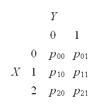
to do this generate variates from a random variable Z with
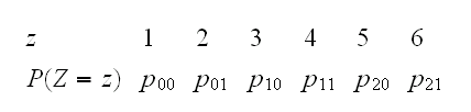
which we can do using the sample command. Then just recode: Z=1→X=0,Y=0, Z=2→X=0,Y=1,..,Z=6→X=2,Y=1
Example this gets a little harder if X or Y take infinitely many values: generate data from (X,Y) with joint pmf f(x,y)=(1-p)2px, x,y {0,1,..}, y≤x, and 0<p<1. Again we need to turn (X,Y) into a one-dimensional r.v Z. Let's use the following coding scheme:
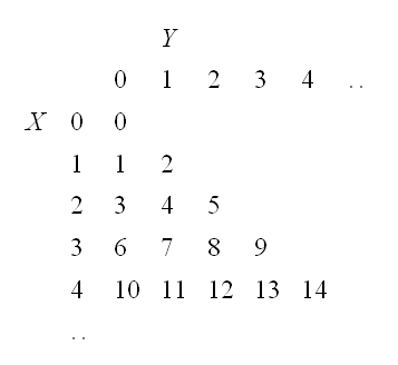
how do we get from (X,Y) to Z and vice versa?
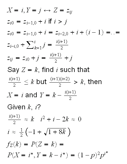
to sample from Z we could use the sample command, except that Z takes infinitely many values. We deal with that by finding k such that P(Z>k)<10-5. All of this is implemented in
sim3()
Example say we want to generate data from a continuous rv (X,Y) with f(x,y)=8xy, 0≤x<y≤1.
For this might use the accept-reject algorithm again. We can generate data (U1,U2) uniform on 0≤x<y≤1 by generating (U1,U2) on [0,1]2 but only using it of U1<U2 . Then of course g(x,y)=2 if 0≤x<y≤1 and

implemented in
sim4(1)
Again the question on how to make sure our algorithm generates the right data. One check is to look at the marginals:
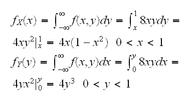
sim4()
draws the histograms of the marginals with these densities. Note, though, that this is no guarantee because the marginals do not determine the joint distribution.
Another idea is to generate the data from conditional distributions:
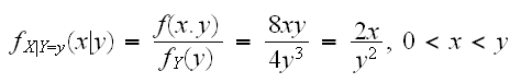
So we can first generate Y and then X|Y=y as follows: Y~Beta(4,1), Z=Beta(2,1) and X=YZ
implemented in
sim4(2)
Simulation Error
Example Say we have the following: Xi~N(0,1) i=1,..,N and M =max{Xi}We want to know E[M] for n=106.
This is simple, see
sim5()
but this turns out to be very slow, on a standard PC it takes about 2 hours if we use n=1000 runs. Given that we cannot do as many as we like, our estimate will have some "simulation error". How large is it? In sim5dat we have the result of one such run. A histogram shows that the "variates" (almost have a normal distribution, so 95% CI is
mean(sim5dat)+c(-1.96,1.96)*sd(sim5dat)/sqrt(1000)
alternatively we can find
sort(sim5dat)[c(25,975)]
Say we want to know P(M>5.05). This we can estimate with
length(sim5dat[sim5dat>5.05])/1000
as 0.022. What is the error in this estimate? Now if we set Yi=I[Mi>5.05] Yi~Ber(p) where p=P(M>5.05) so a 95% CI for p is given by
0.022±1.96√(0.022*0.978/1000) or (0.0129, 0.0311)
Having some idea of what the "simulation error" is usually quite important.