Now if we want to test this in the standard fashion we need to decide on how often we have to flip the coin. This will depend on three things:
• How unfair do we think the coin might be?
• what type I error do we want to use?
• what power do we want our test to have?
say we decide to use the usual 5%, we want a power of 95% and we want to distinguish p=0.5 from p=0.55, then
power.prop.test(p1=0.5,p2=0.55,power=0.95, alternative = "one.sided")
tells us we need a sample size of 2157.
So now we sit down and flip a coin 2157 times. But this gets boring after a while, and so every 100 flips we just perform the hypothesis test
H0: p=0.5 vs Ha: p>0.5
This is done in
coinflips()
Now though it seems we could reject the null hypothesis much earlier, usually already with 200 or 300 flips.
What is going on? To begin with, we have another case of simultaneous inference (here 22 tests). What we need is a procedure that allows for this ongoing testing while keeping the overall type I and type II errors fixed. This is done by sequential analysis.
The most famous method here is called Wald's SLRT (sequential likelihood ratio) test. As the name says, it is based on the likelihood ratio statistics. It also uses one of the famous theorems in Stochastic processes, which says that if N is an integer valued random variable, X1,. X2, .. are iid rv's and
SN=X1+..+XN
then E[SN]=E[N]E[X1]
This of course is Wald's theorem, which he invented to make the SLRT test work.
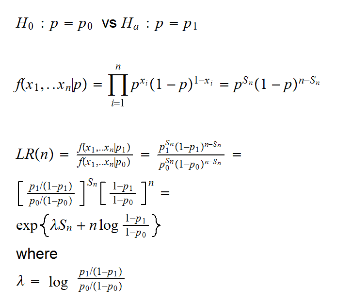
Say we want to test the simple vs simple hypothesis
is the odds ratio.
The test now works as follows: at each step we have the following decisions:
If LR(n)<B, stop and "accept" H0
If LR(n)<A, stop and "accept" Ha
If B<LR(n)<A, take another sample
for A and B Wald suggested
A=(1-β)/α
B=β/(1-α)
Usually the test is done comparing the decision boundaries with Sn. They are
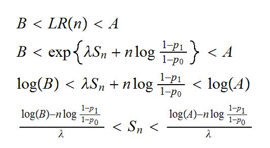
These are drawn in coinflips(2).
How well does this work? In
coinflips(3)
we run the simulation 1000 times. As we can see, it takes on average only 1500 flips to reject the null with a probability of 95%, compared to the 2157 for the fixed sample size experiment.
Now though let's do it one observation at a time:
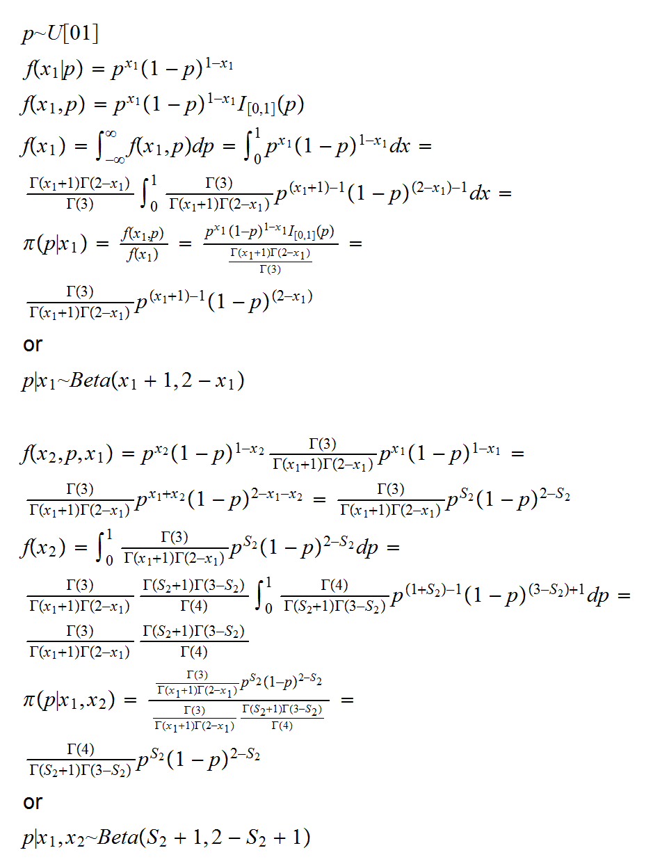
and so we find that the posterior distribution is the same, whether we do the analysis sequencially or with a fixed sample size!
This is often cited as one of the main advantages of a Bayesian analysis over a frequentist one: there is in general no distinction between a fixed sample size and a sequential analysis.