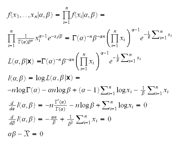
Example Say we have a sample X1,..,Xn from a Gamma(α,β) distribution and we want to estimate α and β. A popular way to do this is using the method of maximum likelihood:
so we see that this amounts to solving a system of nonlinear equations. There is no explicit solution to this problem, which means we have to do it numerically.
Example say f(x)=x5-x4+1. We want to find the roots of f. Now f'(x)=5x4-4x3=x3(5x-4), so f has extrema at x=0, 4/5. f goes to -∞ as x→-∞ and f goes to ∞ as x→∞, so f has a maximum at (0,1) and a minimum at (0.2, 0.9987) Therefore f has a unique zero in (-∞,0). Or instead of the math do
curve(x^5-x^4+1,-1,1.5)
How can we find the root between -1 and 0? Idea:
1) find L such that f(L)<0
2) set H=0, so f(L)<0 and f(H)>0 therefore there is an x such that f(x)=0 and L<x<H.
3) set M=(L+H)/2. if f(M)<0 the root is in (M,H), so set L=M. if f(M)>0 the root is in (L,M) so set H=M
repeat part 3 until H-L<Acc
root.ex()
runs the argorithm, draws the graph and shows the iterations.
For this specific problem of roots of polynomials there is actually an R function buit in:
polyroot(c(1,0,0,0,-1,1))
For general function in one dimension we have
uniroot(f,c(-1,0))
Of course finding the maximum or minimum of a function often means finding the roots of the derivative of the function, although in Statistics minima and maxima often occur at the boundaries as well.
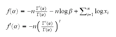
Example back to example at the beginning. let's simplify a bit and assume that β is known, so we need to find the root of d/dα l(α)=0.
gamma.mle(1,alpha=..)
draws the log-likelihood curve and its derivative, called ll.prime. Note that R has some functions already built in: lgamma is the log of the gamma function and digamma is its derivative. As we see the derivative is a decreasing function of alpha, so the bisection algorithm is
1) set L=0
2) set L=L+1, if alpha.p(L)<0 goto 3, otherwise to 2
3) set H=L, L=L-1
4)
set M=(L+H)/2. if alpha.p(M)<0 the root is in (L,M), so set H=M otherwise set L=M
repeat 4) until H-L<Acc
done in
gamma.mle(2)
This is clearly the most important of the general purpose root-finding algorithms, as the name says it goes all the way back to the invention of Calculus by Isaak Newton. It is essentially this:
1) pick a starting point x1
2) xn+1 = xn - f(xn)/f'(xn)
Note: if the algorithm converges to some x we have x=x-f(x)/f'(x) or f(x)=0
Sometimes it is better to use xn+1 = xn - λnf(xn)/f'(xn) for some (predetermined) sequence λn in order to "slow down" or "speed up" the convergence.
Example f(x)=x5-x4+1
root.ex("newton")
Example back to the gamma example. Now we have
Again we get lucky because the second derivative of the log-gamma function is already implemented in R, called trigamma. One problem is that we need a starting point for the algorithm. Note that if X~Γ(α,β), then E[X]=αβ or α=E[X]/β~X̄/β. Now see
gamma.mle(3)
The advantage of Newton-Raphson is that it is very fast. It's problem, though, is it often needs a good starting point or it will not converge. To begin with, if we start at a point where f'(x) is very small, xn+1 will be very far away:
Example f(x)=x1/3. This has a root at 0, but f'(x)=x-2/3/3 and so
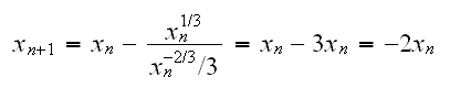
so for any point xn≠0 the next iteration is twice as far from 0!
Here is an example for another possible problem:
Example f(x)=x3-2x+2, so f'(x)=3x2-2. Say we start at x0=0, then
x1=0-f(0)/f'(0)=-2/(-2)=1
x2=1-f(1)/f'(1)=1-1/(-1)=0
and so the algorithm will just jump from 0 to 1 to 0 to 1 ...
Example back to the gamma example. Usually it is not enough to find a point estimate, we also want some idea of the error in the estimate, usually in the form of an interval estimate. How can we do that? According to the large sample theory of maximum likelihood we know that
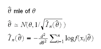
where In is the observed Fisher information number. But it is also the negative of the second derivative of the log-likelihood function, evaluated at the mle. So a 95% CI for α is given by mle±1.96/√-ll.2prime(mle), see again
gamma.mle(3)
Let's see whether this find the correct intervals:
z=matrix(0,1000,3)
for(i in 1:1000) z[i,]=gamma.mle(3,alpha=2.5,Show=F)
(length(z[z[,2]>2.5,1])+length(z[z[,3]<2.5,1]))/1000
So one advantage of using Newton-Raphson is that we get error estimates "for free", as part of the calculations.
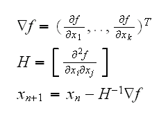
Multidimensional Newton-Raphson
say we have a function f from Rn into R, and we want to find its extrema. Then the Newton-Raphson algorithm is
Example find the maximum of
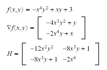
root.ex("3D",A=0.1,start=c(0.1,0.1,0.1))
Example And again the gamma example, this time for both α and β. We have
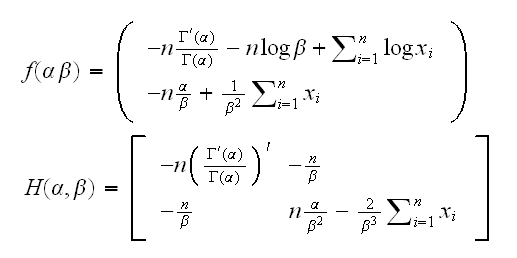
How about the starting point? Note
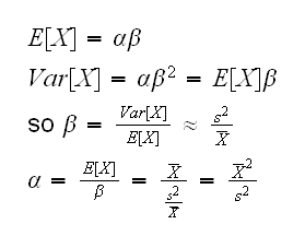
implemented in
gamma.mle(4)
Notice that we did not make use of the fact that the second equation is actually not non-linear but simplifies to β=X̄/α. This we can use in a "hybrid" type of method:
1) find the next guess for α using Newton-Raphson
2) find the next guess for β with X̄/α
done in
gamma.mle(5)
This is a bit slower than the 2-dim Netwon-Raphson but is easier to implement and likely more stable.
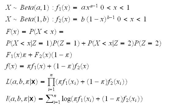
Example: We have observations X1, ..,Xn which are independent. We know that our population is made up of two groups (Men - Women, say) and each observation comes from one or the other group but we don't know which. Observations from group 1 have a Beta(a,1) distribution, those from group 2 a Beta(1,b). We want to estimate the parameters using the method of maximum likelihood.
What we have here is called a mixture distribution. Say that the proportion of members of group 1 in the population is π. Let's introduce a latent (unobserved) r.v. Zi, which is 1 if observation Xi comes from group 1, and 2 if it comes from 2. Then
To find the mle we need to find the partial derivatives and solve the resulting system. To simplify the calculation let's supress any mention of the xi's and introduce some notation:
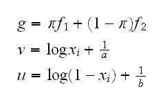
Now
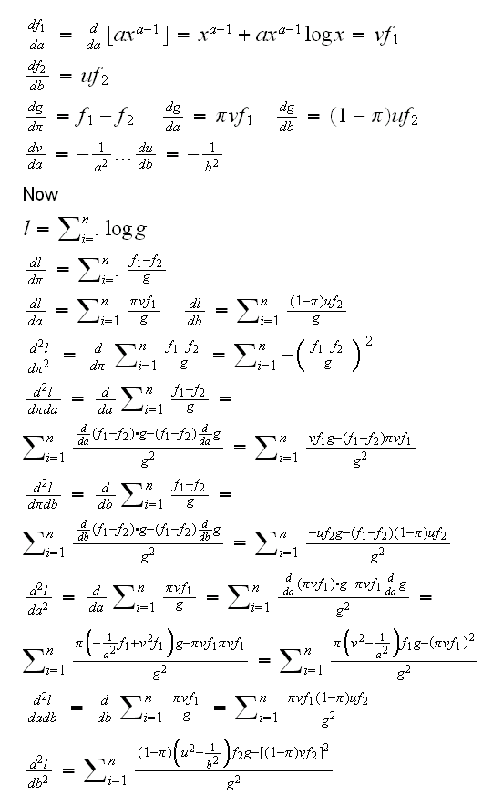
This is implemented in
mixmle()
Notice that here the algorithm can fail quite badly, even if we start at a very good point (the "correct" point used to generate the data). For example, consider the data in mix.ex. This was generated with the command
mix.ex=c(rbeta(2500,2,1),rbeta(2500,1,4))
It turns out that the mle's are 0.4985, 1.9786, 3.9631 which has log-likelihood=232.06. Now if we run
mixmle(x=mix.ex,start=c(0.5,2,4))
it actually diverges. Even
mixmle(x=mix.ex,start=c(0.4985, 1.9786, 3.9631))
does! In mixmle we have the option to keep any of the three parameters fixed, and find the maximum for the others. See
mixmle(x=mix.ex,start=c(0.4985, 1.9786, 4),which=c(1,3))
and all its variations show that as long as we fit just one or two parameters the routine converges fine.
We will soon find an algorithm that works quite a bit better for this type of problem.
Let's have another look at the dataset mix.ex. Say we want to find a 95% Ci for the mixing ratio π. Again we can use the large sample theory of maximum likelihood estimators. In the notation here the observed information number is H[1,1]. So
mixmle(x=mix.ex,start=c(0.4003, 2.537, 2.39524),doH=T)
shows H[1,1]=-11651.3762, so the standard deviation of the mle of π is 1/√11651= 0.009 and so a 95% CI is 0.4985±1.96*0.009 or
(0.481, 0.516)
For a and be, respectively. we find
1.9786±1.96/√243 or (1.853, 2.104)
3.9631±1.96/√66.9 or (3.72, 4.203)
Caution: this is not as simple as it looks here, there are several complication factors: first there is the usual issue of simultaneous inference, second there is the question of how to extract an interval from the likelihood surface. Say we have two parameters, then the joint distribution of the mle's is approximately bivariate normal. In the above we extracted the intervals without consideration of the correlations. In the next graph we draw the contourplot of a likelihood surface with 95% probability:
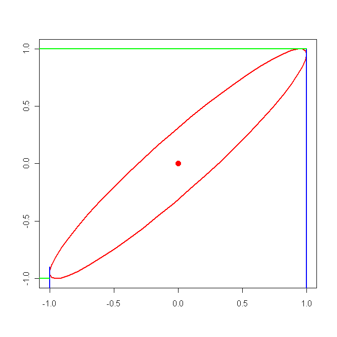
clearly we will get intervals that are actually
a bit to large. In our case the off-diagonal elements of H are small compared the diagonal ones, so our intervals should be quite good.
Example find
int.ex(1,4)
This still works in 2 dimensions:
Example find
int.ex(2)