but this is the same as the maximum likelihood equation for X~Beta(a,1) where we only count those xi's where zi=1. In other words, if we knew the zi's, estimating a and b would be an easy problem: just find the mle's for groups 1 and 2 separately.
The EM algorithm seems at first to solve a very specific problem but it turns out to be quite useful in general
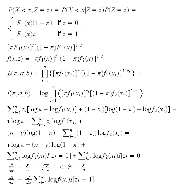
Example Let's return to the mixture model we considered earlier: Y1~Beta(a,1), Y2~Beta(1,b), Z~Ber(π) and X=(1-Z)Y1+ZY2 Let's assume for the moment that in addition to the X1, .., Xn we also observe Z 1, .., Z n where Z=1 if observation is from group1, Z=0 if group 2. Let y=∑zi be the number of observations from group 1, then
but this is the same as the maximum likelihood equation for X~Beta(a,1) where we only count those xi's where zi=1. In other words, if we knew the zi's, estimating a and b would be an easy problem: just find the mle's for groups 1 and 2 separately.
On the other hand,
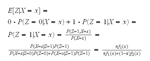
so if we knew the parameters a and b we could estimate each of the zi's.
Note that if X~Beta(a,1) we have
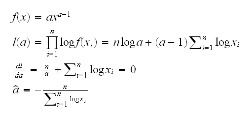
Of course πf1(x)/(πf1(x)+(1-π)f2(x))  (0,1), so we need to replace the zi's with weights wi and the formulas become
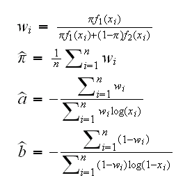
This is then the basic idea of the EM algorithm:
• in the M(aximization) step assume you know the weights w 1,..,wn and estimate the parameters via mle
• in the E(stimation) step use these parameters to estimate the w 1,..,wn.
See
em1()
for an implementation. Notice a nice feature of the EM algorithm: in each step it finds a point which is at least as good as the last one.
How well does this work? Let's do a little checking: generate some data, use em1 to find the mle, and find the log-likelihood for some points around the mle:
x=c(rbeta(500,2,1),rbeta(500,1,2))
p=em1(x=x,start=c(0.5,2,2),Show=F)
p
em1.test(x,p[1:3])
The EM algorithm was originally invented by Dempster and Laird in 1977 to deal with a common problem in Statistics called censoring: say we are doing a study on survival of patients after cancer surgery. Any such study will have a time limit after which we will have to start with the data analysis, but hopefully there will still be some patients who are alive, so we don't know their survival times, but we do know that the survival times are greater than the time that has past sofar. We say the data is censored at time T. The number of patients with survival times >T is important information and should be used in the analysis. If we order the observations into (x1, .., xn) the uncensored observations (the survival times of those patients that are now dead) and (xn+1, .., xn+m) the censored data, the likelihood function can be written as
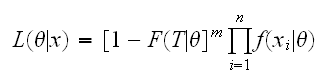
because all we know of the censored data is that P(Xi>T)=1-F(T|θ)
If we had also observed the survival-times of the censored patients, say z=(zn+1, .., zn+m) we could have written the complete-data likelihood
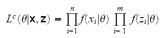
and again we can use the EM algorithm to estimate θ:
• in the M step assume you know the z1,..,zn and estimate θ.
• in the E step use θ to estimate the z1,..,zn
Example Say Xi~Exp(θ), we have data X 1, .., Xn and we know that m observations were censored at T. Now
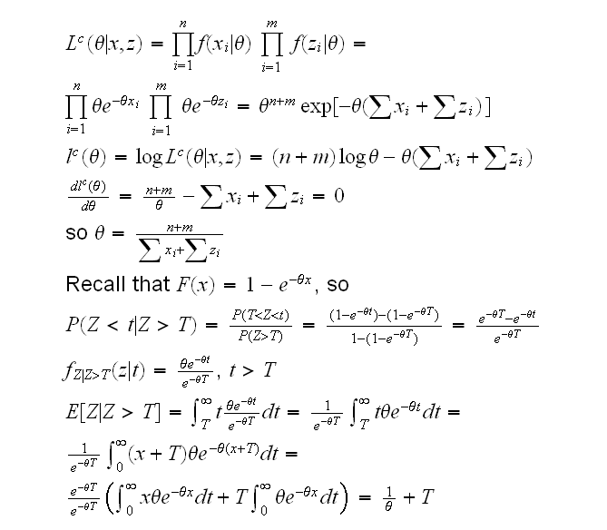
Of course E[Z|Z>T]=T+1/θ also follows immediatley from the memory-less property of the exponential!
so the EM algorithm proceeds as follows:
• in the M step assume you know the z1,..,zn and estimate θ=1/mean({x1, .., x n,zn+1, .., zn+m}).
• in the E step use θ to estimate the z1,..,zn =1/θ+T
em2()
The application of the EM algorithm to the mixture problem above is to the case where every observation is censored, because we don't know any of z's!