It is useful to do a little bit of probability theory and theoretical statistics, especially decision theory. Let X Rn denote a real-valued random input vector and Y be an output vector, with joint probability distribution P(X,Y). We seek a function f(X) for predicting Y given values of input X. Decision theory requires a loss function L(Y,f(X)) for penalizing errors in prediction.
Let's take a moment to digress and assume that Y is a real-valued output vector. Then by far the most common error function is square error loss
L(Y,f(X)) = (Y-f(X))2
This leads to a criterion for choosing f, the expected prediction error:
EPE(f) = EL(Y,f(X)) = E(Y-f(X))2 = ∫(y-f(x))2P(dx,dy)
Using a well-known formula for conditional expectations we have
EPE(f) = EXEY|X([Y-f(X)]2|X)
and so it suffices to minimize EPE pointwise:
f(x) = argmincEY|X([Y-c]2|X=x)
The solution is f(x) = E(Y|X=x), the conditional expectation. So the best prediction for Y at any point X=x is the conditional mean (if we agree on square error loss).
Now let's assume that f(x) is approximately linear, that is f(x) = xTβ Plugging this linear model for f(x) into EPE and differentiating we can solve for β theoretically and we find
β = [E(XXT]-1E(XY)
so we have just found a justification for least-squares regression within the Bayesian framework.
Let's get back to the discrimination problem. Here the "response" Y is a discrete variable, namely Y=k if the observation belongs to the kth class. In such a situation the loss function is a matrix. Say we observe X=x and estimate the class to be T(x){1,..,k}. The loss function is then a k by k matrix L. L is 0 on the diagonal (no loss if we are correct in our assignment) and nonnegative elsewhere, where Lij is the price paid if we classify an observation from class i wrongly as class j. Quite common is to use zero-one loss where Lij = 1 if i≠j. Now the expected prediction error is
EPE = ELT(X)
As before we can condition and get
EPE = EX∑LkT(X)P(k|X)
and again we can minimize pointwise to get
T(x) = argminyY∑LkyP(k|X=x)
If we use 0-1 loss this simplifies to
T(x) = argminyY[1-P(y|X=x)]
or
T(X) = k if P(k|X=x] = maxy P(y|X=x)
This seems very reasonable: assign an observation to class k if class k has the highest posterior probability, given X=x. This rule is called the Bayes classifier. The miss-classification rate of the Bayes classifier is called the Bayes rate, and is the best achievable rate.
Note that the k-nearest neighbor method directly approximates this solution, where we estimate the unknown posterior probability by the majority vote of the neighboring observations.
Suppose we have a two-class problem, and we used the linear regression approach with a dummy response variable y, followed by squared-error loss estimation. Then
f(X) = E(Y|X) = P(Y=1|X)
because expectations of indicator variables are probabilities. And so again we see that this method also tries to approximate the Bayes classifier!
The Curse of Dimensionality (Bellman, 1961)
As a general prinicple, problems that are easy in low dimensions get very hard in high dimensions. As Bellman pointed out, our everyday intution often fails in high-dimensions spaces. Here is one classical example:
Consider the nearest-neigbor method for inputs x uniformly distributed in a p-dimensionsl unit hypercube, that is x = (x1, .. ,xp), xk~U[0,1] and xi xj if i≠j. Say instead of Euclidean distance we use hypercubical neighborhoods, and for a target point we want to find a neighborhood that captures a fraction r of the observations. For p=2 this is illustrated in curse.fun()
Now the expected edge length will be ep(r)=r1/p. In ten dimensions e10(0.01)=0.63, so to capture 1% of the data the neighborhood has to cover 68% of the range of each input variable!
Here is another example: Consider N data points uniformly distributed in a p-dimensional unit ball centered at the origin. Suppose we consider a nearest neigbor estimate at the origin. The median distance from the origin to the closest data point is given by

Now d(5000,10)=0.52, so most data points are closer to the boundary of the sample space than to any other data point!
One consequence of all this is that classification in high dimensions is very difficult. Especially nearest neighbor methods are no longer useful.
LDA and QDA
The decision theory above showed that we need to know the class posteriors P(Y|X) for optimal classification. Suppose fk(x) is the class-conditional density of X in class Y=k, and let πk be the prior probability of class k, with ∑πk=1. A simple application of Bayes' formula gives:
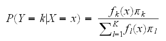
and we see that for classification having fk(x) is almost equivalent to having P(Y=k|x).
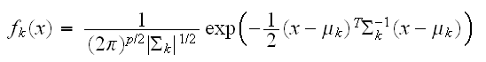
A number of methods are based on estimating the class-conditional densities. One popular approach called linear and quadratic discriminant analysis assumes these to be Gaussian densities, that we assume
Linear discriminant analysis (LDA) assumes that all the classes have the same variance-covariance matrix σk = σ. In comparing two classes k and l it is sufficient to look at the log-odds ratio and we see
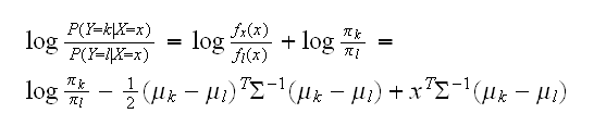
a linear equation in x. This linear log-odds function implies that the decision boundary between classes k and l is linear in x; in p dimensions it is an affine plane (a hyperplane which does not go through the origin)
If there are only two classes this can be shown to be the same method as our "lm". If there are more than two they are not.
If the σk are not all the same the math becomes more complicated but is still doable, and the resulting method is similar to our "quadratic" method.
R has both methods implemented, and we use them in
class2.fun(1,"lda")
on our three examples.
Classification Trees
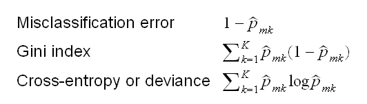
We have previously discussed regression trees. These models can also be used to do classification. The only changes needed in the tree algorithm concern the criteria for splitting nodes and pruning trees. For regression trees we used the square-error node impuity measure Qm(T). Here for a node m representing a region Rm with Nm observations let
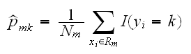
be the proportion of class k observations in node m. We classify the observations in node m to class k(m) which has the highest proportion. Then different measures of node impurity include:
In R we again use the routine rpart, with the argument method="class". This is implemented in
class3.fun(1)
for our three examples.