Some Applications of the Bootstrap

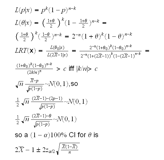
Let's begin with a standard statistical analysis of this problem. That means we first need a probability model for this experiment. Here this is clearly as follows: let X_i=1 if vote is for A, 0 if it is for B, then X_i~Ber(p). We can assume that X₁, .., X_n are independent. The parameter of interest is the difference in proportions θ=p-(1-p)= 2p-1.

Frequentist Analysis: we already know that the mle of p is X̄, so the mle of θ is 2X̄-1 , here 2·0.523-1= 0.046.

Of course if θ=2p-1 we have p=[1+θ]/2, so


and for our numbers we get the interval (-0.016, 0.108), see

diffprop().

Bayesian Analysis: Our parameter is θ with values in [-1,1], so we need a prior with values in this interval. For p we usually use Beta(α,β), and then we have

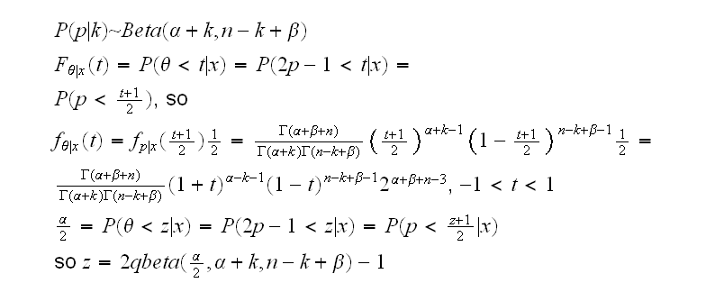
which yields the interval (-0.016, 0.108) using α=β=1, again done in

diffprop()

Now how about using the bootstrap? Done in

lead.boot()

Example (from "An Introduction to the Bootstrap" by Bradley Efron and Robert Tibshirani) The data is the thicknesses (espesor) in millimeters of 485 Mexican stamps (sello) printed in 1872-1874, from the 1872 Hidalgo issue. her is one of them:

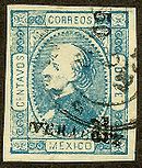
It is thought that the stamps from this issue are a "mixture" of different type of paper, of different thicknesses. Can we determinse from the data how many different types of paper were used?

As a first look at the data let's draw several histograms, with different bins. This is done in

stamps.fun(1)

It seems there are at least two and possibly as many as 6 or 7 "peaks" or "modes".

Here we are using the histogram as a "density estimator", that is we visualize the "top" of the histogram as a density. In

stamps.fun(2)

we draw just that "top".

The main problem with this is that the true density is continuous but the histogram is not smooth. Instead we should use a "nonparametric density estmator" A popular choice is a kernel density estimator:

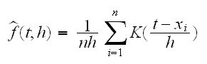
where h is called the bandwidth (equivalent to the binwidth of histograms) and K is called the kernel function. A popular choice for K is the density of a standard normal rv. In

stamps.fun(3)

we draw four different curves for different values of h. As we can see, the smaller h gets the more ragged the curve is.

It is clear that the number of modes depends on the choice of h. It is possible to show that the number of modes is a non-increasing function of h.

Let's say we want to test H₀: number of modes=1 vs. H_a: number of modes>1 Because the number of modes is a non-increasing function of h there exists an h₁ such that the density estimator has one mode for h<h₁ and two or more mode for h>h₁. Playing around with

stamps.fun(4,h=..)

we can see that h₁~0.0068.

Is there a way to calculate the number of modes for a given h? here is one:

• calculate y_i=fhat(t_i;h) on a grid t₁,..t_k
• calculate z_i=y_i-1-y_i and note that at a mode z will change from positive to negative.
• # of modes = ∑I[z_i>0 and z_i+1<0]

In

stamps.fun(5,want.mode=..)

we "automate the process to find the largest h which yields want.mode modes. It uses the "bisection algorithm".

So, how we can test H₀: number of modes=1 vs. H_a: number of modes>1? Here it is:

• draw B bootstrap samples of size n from fhat(.,h₁)
• for each find h₁star, the smallest h for which this bootstrap sample has just 1 mode
• approximate p-value of test is #{h₁star>h₁}/B

Notice we don't actually need h₁star, we just need to check if h₁star>h₁, which is the case if fhat_xtar(.,h₁) has at least two modes.

Note that we are not drawing bootstrap samples from "stamps" but from a density, fhat. This type of bootstrap is called a smooth bootstrap.

How do we draw from fhat? Let y₁star,..,y_nstar be a bootstrap sample from the data, and set

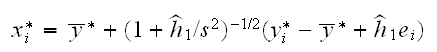
where s² is the variance of the data and &ε_i are standard normal rv's. The term (1+h₁star/s²) insures that the bootstrap sample has the same variance as the data, which turns out to be a good idea.

It is done in

stamps.fun(6,want.mode=1)

Finally we can test for 2 modes vs more than 2 modes etc, in a similar fasion. The results are shown here:

# of modes	hm	p-value
1	0.0068	0.00
2	0.0032	0.29
3	0.0030	0.06
4	0.0029	0.00
5	0.0027	0.00
6	0.0025	0.00
7	0.0015	0.46
8	0.0014	0.17
9	0.0011	0.17

So there are certainly more than one mode, with a chance for as many 7.

Example In the dataset boot1.ex we have a sample of size 150 from a distribution with density

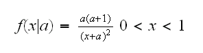
and we want to find a 95% CI for the parameter a. Would an interval based on the large sample theory of mle's or a bootstrap based interval be better?

First we need to find the mle:

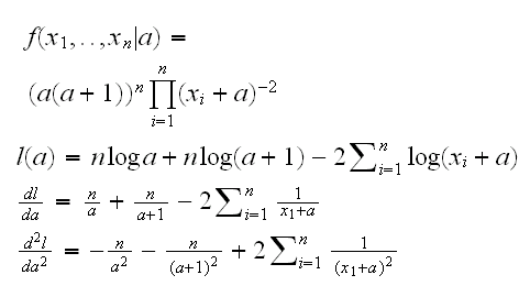
In

boot1(boot1.ex)

we use Newton-Raphson to find the mle and its large-sample 95% CI: (0.28, 0.63) and we find the percentile Bootstrap interval to be (0.34, 0.67) .

So which is better? In

boot1.test()

we run a little simulation which shows that both have just about the right coverage.