Random Variables
A **random variable** (r.v.) X is set-valued function from the sample space into .
Example 1: We roll a fair die, X is the number shown on the die
Example 2: We roll a fair die, X is 1 if the die shows a six, 0 otherwise.
Example 3: We roll a a fair die until the the first "6", X is the number of rolls needed.
Example 4: We randomly pick a time between 10am and 12 am, X is the minutes that have passed since 10am.
There are two basic types of r.v.'s:
If X takes countably many values, X is called a **discrete** r.v.
If X takes uncountably many values, X is called a **continuous** r.v.
There are also mixtures of these two.
In Examples 1, 2 and 3 above X is discrete, in Example 4 X is continuous.
There are some technical difficulties when defining a r.v. on a sample space like , it turns out to be impossible to define it for every subset of  without getting logical contradictions. The solution is to define a **σ-algebra** on the sample space and then define X only on that σ-algebra. We will ignore these technical difficulties.
Almost everything to do with r.v.'s has to be done twice, once for discrete and once for continuous r.v.'s. This separation is only artificial, it goes away once a more general definition of "integral" is used (Rieman-Stilties or Lebesgue)
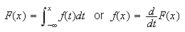
(Commulative) Distribution Function
The distribution function of a r.v. X is defined by P(X$\le$x)  x  
Example 1: say x=2.2, then P(X$\le$x) = P(X$\le$2.2) = P({1,2}) = 2/6 =1/3
Example 4: say x=67.5, then P(X$\le$67.5) = P(we chose a moment between 10am and 11h7.5min am) = 67.5/120 = 0.5625
Some features of cdf's:
1) cdf's are standard functions on 
2) 0$\le$F(x)$\le$1 x
3) cdf's are non-decreasing
4) cdf's are right-continuous
5)

**Example** : find the cdf F of the random variable X in Example 3 above.
Solution: note X{1,2,3,...}
let A_i be the event "a six on the i^th roll", i=1,2,3, .... Then
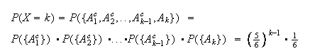
and
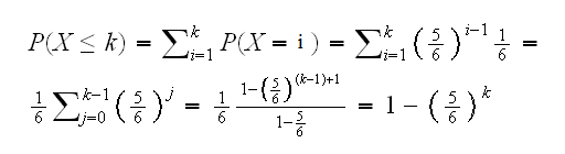
so for k$\le$xProbability Mass Function (density) - Probability Density Function (pdf)
The probability mass function (density) of a discrete r.v. X is defined by f(x) = P(X=x)  x  
**Example** : the pdf of X in Example 3 is given by f(x) = 1/6*(5/6)^x-1 if x{1,2,..}, 0 otherwise.
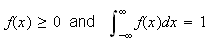
Note that it follows from the definition and the axioms that for any density f we have
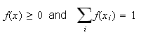
The function f is called the probability density function of the continuous random variable X iff
Again it follows from the definition and the axioms that for any pdf f we have
**Example**: Show that f(x)=λexp(-λx) if x>0, 0 otherwise defines a pdf, where λ>0
Solution: clearly f(x)$\ge$0 for all x.

This r.v. X is called an exponential r.v. with rate λ.
Random Vectors
A random vector is a multi-dimensional random variable.
**Example** : we roll a fair die twice. Let X be the sum of the rolls and let Y be the absolute difference between the two roles. Then (X,Y) is a 2-dimensional random vector. The joint density of (X,Y) is given by:
| **X\Y** |
**0** |
**1** |
**2** |
**3** |
**4** |
**5** |
| **2** |
1 |
0 |
0 |
0 |
0 |
0 |
| **3** |
0 |
2 |
0 |
0 |
0 |
0 |
| **4** |
1 |
0 |
2 |
0 |
0 |
0 |
| **5** |
0 |
2 |
0 |
2 |
0 |
0 |
| **6** |
1 |
0 |
2 |
0 |
2 |
0 |
| **7** |
0 |
2 |
0 |
2 |
0 |
2 |
| **8** |
1 |
0 |
2 |
0 |
2 |
0 |
| **9** |
0 |
2 |
0 |
2 |
0 |
0 |
| **10** |
1 |
0 |
2 |
0 |
0 |
0 |
| **11** |
0 |
2 |
0 |
0 |
0 |
0 |
| **12** |
1 |
0 |
0 |
0 |
0 |
0 |
where every number is divided by 36.
all definitions are straightforward extensions of the one-dimensional case.
**Example** : for a discrete random vector we have the density f(x,y) = P(X=x,Y=y)
Say f(4,0) = P(X=4, Y=0) = P({(2,2)}) = 1/36 or f(7,1) = P(X=7,Y=1) = P({(3,4),(4,3)}) = 1/18
**Example** Say f(x,y)=cxy, 0$\le$xConditional R.V.'s
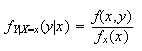
let (X,Y) be a discrete r.v. with joint density f(x,y) and marginals density f_X and f_Y. For any x such that f_X(x)>0 the conditional density f_Y|X=x(y|x) is defined by
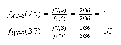
**Example**: find f_X|Y=5(7|5) and f_Y|X=3(7|3)
For continous r.v. everything works the same:
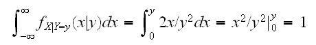
**Example** Find f_X|Y=y(x|y)
f_X|Y=y(x|y) = f(x,y)/f_Y(y) = 8xy/4y^3 = 2x/y^2, **0$\le$x$\le$y**. Here y is a fixed number!
Again, note that a conditional pdf is a proper pdf:
Note that a conditional density (pdf) requires a specification for a value of the random variable on which we condition, something like f_X|Y=y. An expression like f_X|Y is not defined!
Independence
Two r.v. X and Y are said to be independent iff f_X,Y(x,y)=f_X(x)*f_Y(y)
**Example** : in the example above we found f_X,Y(7,1) = 1/18 but f_X(7)*f_Y(1) = 1/6*10/36=5/108, so X and Y are not independent
Mostly the concept of independence is used in reverse: we assume X and Y are independent (based on good reason!) and then make use of the formula:
Say we use the computer to generate 10 independent exponential r.v's with rate λ. What is the probability density function of this random vector?
We have f_X_i(x_i)=λexp(-λx_i) for i=1,2,..,10 so
f_(X_1,..,X_10)(x_1, .., x_10) =
λexp(-λx_1) *..* λexp(-λx_10) = λ^10exp(-λ(x_1+..+x_10))
Notation: we will use the notation X  Y if X and Y are independent