Ordinary Linear Regression

Example Consider the the dataset hubble. In 1929 Edwin Hubble published a paper showing a relationship between the distance and radial velocity away from Earth of "extra-galactic nebulae" (galaxies). His findings revolutionized astronomy. The "Hubble constant," the slope of the regression of velocity (Y) on distance (X), is still a subject of research and debate. The data here are those Hubble published in his original paper.

Question: If it is true there is a linear relationship between Velocity (Y) and Distance (X), what is the slope of the line?

If there is a linear relationship, there exist β₀ and β₁ such that

Y_i=β₀+β₁X_i+ε_i i=1,..,n

where the ε_i are called the residuals.

In the problem above the main task is to find a interval estimate for β₁. In other problems it might be to estimate Y for a specific value of x, to estimate E[Y] for some x, to see whether β₀ or β₁ are zero (or some other value) etc.

Another version of the regression problem is Y_i=β₀+β₁x_i+ε_i i=1,..,n that is the x's are not random but fixed for example the number of car accidents in Puert Rico (Y) by the year (x).

First we need a probability model. Again this will depend on the problem, but an often used is to assume that (X,Y) are bivariate normal with parameters (μ_x,μ_y,σ_x,σ_y,ρ) If we think in terms of predicting Y from a fixed value of X=x, the we need the conditional distribution of Y|X=x, which N(μ_y+ρσ_y/σ_x(x-μ_x),σ_y√(1-ρ₂)). Therefore we have

E[Y|X=x] = μ_y+ρσ_y/σ_x(x-μ_x) = μ_y-μ_xρσ_y/σ_x+ρσ_y/σ_xx

so we find that under this probability model we have a natural linear relationship between X and Y with

β₀=μ_y-μ_xρσ_y/σ_x and β₁=ρσ_y/σ_x

Generally in a regression context the analysis is carried out using the conditional distribution of (Y₁,..,Y_n) given X₁=x₁,..,X_n=x_n., in which case we can consider the x's as fixed and known. the probability model then becomes

Y_i=β₀+β₁x_i+ε_i , ε_i ~N(0,σ), i=1,..,n

Notice that we are assuming equal variance. If this is not reasonable, the analysis is still possible but somewhat more difficult.

First let's find the mle's of β_0, β₁: and σ:

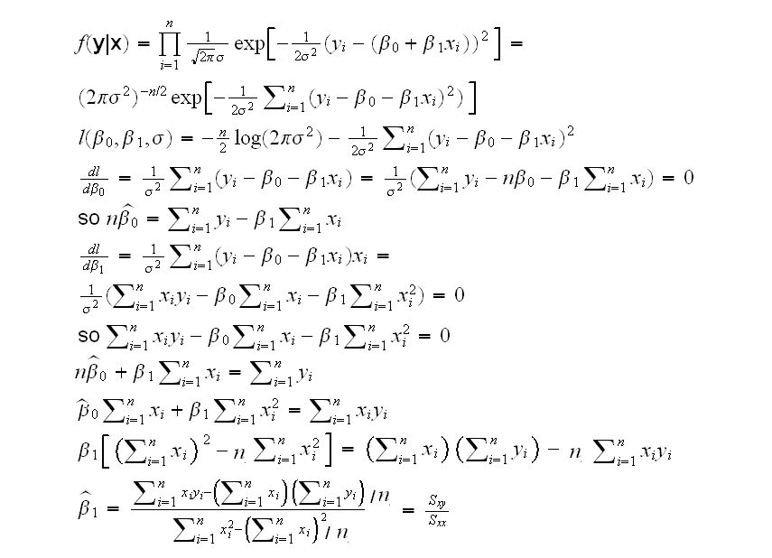
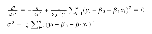
which are of course the standard least squares regression estimates! For σ² we find

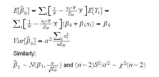
What are the sampling distributions?

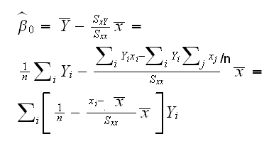
and so β₀ is a linear combination of normal rv's, and therefore normal itself. Moreover

A confidence interval for the slope can be found as follows:

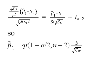
and in hubble.est the 95% CI is calculated to be (298, 610)