The main issue in a Bayesian analysis is always the choice of priors. Here are some of the common methods:
Subjective Prior
In many ways this is was is required by the Bayesian paradigm, namely to find a prior that "encodes" your subjective belief about the parameter.
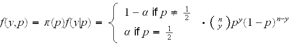
Example let's again the the coin example from before. Here is a very different, but probably more realistic, prior: Before we flip the coin we reason as follows: either the coin is fair, and we think that is most likely the case, or if it is not, we don't have any idea what it might be. We can "encode" this belief in the following prior:
Let δ1/2 be the point mass at 1/2, that is a random variable which always takes the value 1/2, or P(d1/2 = 1/2) = 1. Let U~U[0,1] and let Z~Ber(α). Now
p = Zd1/2 + (1-Z)U
So with probability α p is just 1/2 (and the coin is fair), and with probability 1-α p is uniform on [0,1] (and we don't have any idea what's going on).
This prior is a mixture of a discrete and a continuous r.v. so we will need to be a bit careful with the calculations.
The cdf and the prior "density" are as follows

The joint density of p and y is:
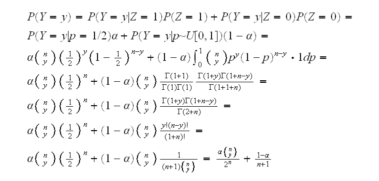
and the marginal distribution of y:
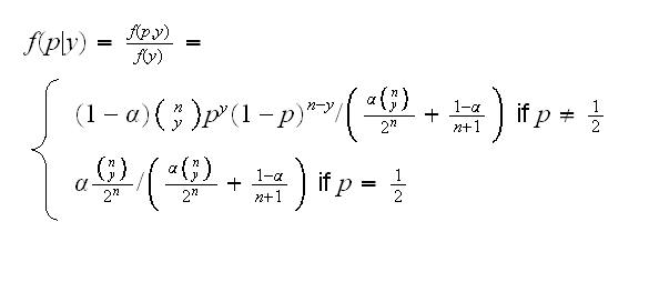
Now we find the posterior distribution of p given y:
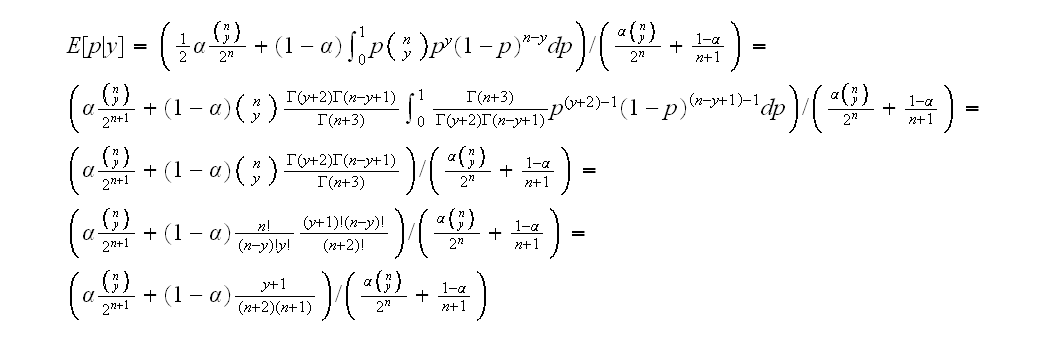
Finally as above we can find the mean of the posterior distribution to get an estimate of p for a given y:
Generally finding a good subjective prior can be done using utility theory.
Conjugate Priors
these are priors which together with the sampling distribution lead to a posterior distribution of the same type as the prior. Here are some examples
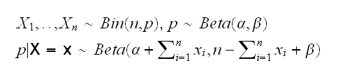
Binomial-Beta
Normal-Normal
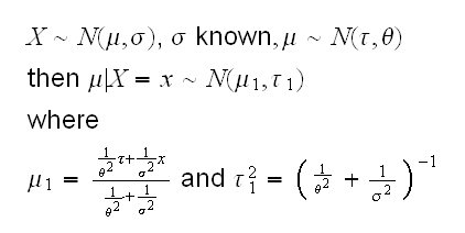
where τ and θ are assumed to be known.
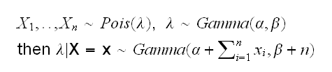
Poisson-Gamma
Non-informative Priors
just what it says, a prior that does not contain any "information" on the parameter.
Example X1, .., Xn~Ber(p), then p~U[0,1] is a non-informative prior.
Example X1, .., Xn~N(μ,1) now μ can be any real number, so a prior has to be a density on the whole real line. But π(μ)=c is not possible because it integrates out to infinity for any c>0!
There are two solutions to this problem:
a) Allow improper priors, that is priors with an infinite integral. This is generally ok as long as the posterior is a proper density:
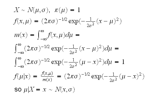
One justification for this is that we usually can express the improper prior as the limit of a sequence of proper priors: we saw already that if X~N(μ,σ) and μ~N(τ,θ), then μ|X=x is again normal. Now

b) A second solution is to think a little more about what "non-informative" really means, Say we have X1, .., Xn iid N(μ,σ) and we want to estimate σ. At first it seems we should use p(σ)=1, σ>0 It turns out, though, that this is not really "competely non-informative" because of the following: say we estimate σ=2.7, then there is small interval (0,2.7) "below" our estimate but a very large interval "(2.7, ∞) "above" it. There is a class of priors that were developed explicitely to express this idea of "complete lack of knowledge" called Jeffrey's priors.
Empirical Bayes
Example say X1, .., Xn~Pois(λ) and λ~Gamma(α,β), then we know that λ|X=x~Gamma(α+∑xi, β+n). But how do we choose α and β? In a subjective Bayesian analysis we would need to use prior knowledge to estimate them. The idea of empirical Bayes is to use the data itself to estimate the "hyper-parameters" α and β. For example, we know that the mean of a Gamma(α,β) is αβ and the variance is αβ2. So we choose α and β as the solutions of the system of non-linear equations
X̅=αβ
s2=αβ2
or
s2=αβ·β=X̅·β
so β=s2/X̅ and α=X̅/β=X̅2/s2
One can go even further and use the empirical distribution function as the cdf of the prior itself. In many ways, though, empirical Bayes goes against the spirit of Bayesian analysis.
These are just some of the methods for finding priors, there are many others.