an→a iff
for every ε>0 there exists an nε such that |an-a|<ε for all n>nε
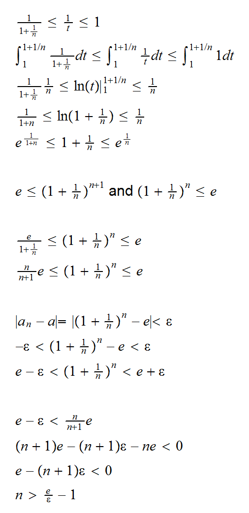
Example say an=(1+1/n)n. Show that an→e
Fix n, and let t be such that 1≤t≤1+1/n. Then
so fix an ε>0. Then if n>e/ε-1 we have |(1+1/n)n-e|<ε, and therefore
(1+1/n)n→e
Things already get a little more complicated if we go to sequences of functions. Here there are two ways in which they can converge:
• Pointwise Convergence: fn(x)→f(x) pointwise for all x S iff for every xS and every ε>0 there exists an nε,x such that |fn(x)-f(x)|<ε for all n>nε,x
• Uniform Convergence: fn(x)→f(x) uniformly for all xS iff for every xS and every ε>0 there exists an nε (independent of x!) such that |fn(x)-f(x)|<ε for all n>nε
and there is a simple hierarchy: uniform convergence implies pointwise convergence but not vice versa
Example say fn(x)=1+x/n, x , S=[A,B] where A<B, f(x)=1, then fn(x)→f(x) uniformly.
|fn(x)-f(x)| = |1+x/n-1| = |x/n| ≤ max(|A|,|B|)/n < ε if n≥max(|A|,|B|)/ε
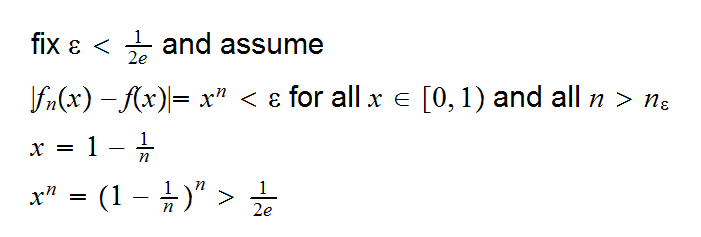
Example say fn(x)=xn , S=[0,1] f(x)=I{1}(x), then fn(x)→f(x) pointwise but not uniformly.
say x<1 then |fn(x)-f(x)| = xn < ε for all n > nε,x = log(ε)/log(x)
say x=1 then |fn(x)-f(x)| = 0 < ε for all n > nε,x = 1
but
Now when we go to probabilities it gets a bit more complicated. Say we have a sequence of rv's Xn with means μn and cdf's Fn, and a rv X with mean μ and cdf F. Then we have:
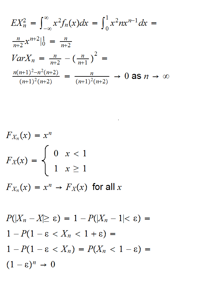
• Convergence in Quadratic Mean Xn→ μ in quadratic mean iff E[Xn]→μ and Var(Xn)→0
• Convergence in Distribution (Law) Xn→X in law iff Fn(x)→F(x) pointwise for all x where F is continuous
• Convergence in Probability Xn→X in probability iff for every ε>0 limn→∞P(|Xn-X|≥ε)=0
• Almost Sure Convergence Xn→X almost surely iff for every ε>0 P(limn→∞|Xn-X|<ε)=1
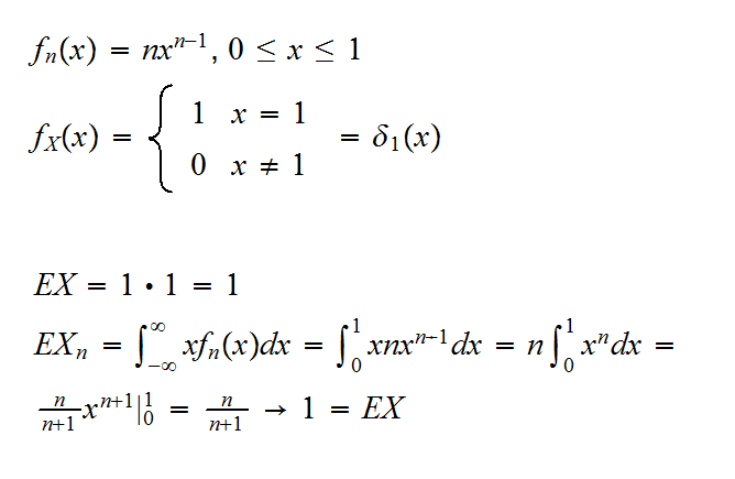
Example Let Xn have density fn(x)=nxn-1, 0<x<1 (X~Beta(n,1)) and let X be such that P(X=1)=1. Then
Unfortunately there is no simple hierarchy between the different modes of convergence. Here are some relationships:
a) convergence in quadratic mean implies convergence in probability.
b) convergence in probability implies convergence in distribution. The reverse is true if the limit is a constant.
c) almost sure convergence implies convergence in probability, but not vice versa
proof (assuming in addition that V(Xi)=σ2 < ∞)
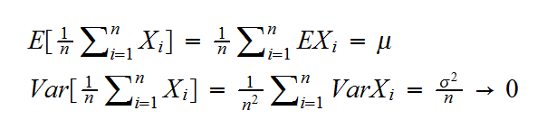
so X̅ →μ in quadratic mean and therefore in probability.
It is best to think of this (and other) limits theorems not as one theorem but as a family of theorems, all with the same conclusion but with different conditions. For example there are weak laws even if the Xn's are not independent, don't have the same mean and don't have even have finite standard deviations.
Let X1, X2, ... be a sequence of independent and identically distributed (iid) r.v.'s having mean μ. Then X̅ converges to μ almost surely
Recall: a random variable X is said to be normally distributed with mean μ and variance σ2 if it has density:
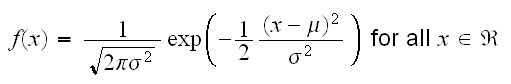
If μ=0 and σ=1 we say X has a standard normal distribution.
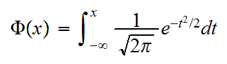
We use the symbol Φ for the distribution function of a standard normal r.v., so
Let X1, X2, .. be a sequence of r.v.'s with means E[Xi]=μi and sd(Xi)=σi. Let X̅n be the sample mean of the first n observations. Then a central limit theorem would assert that
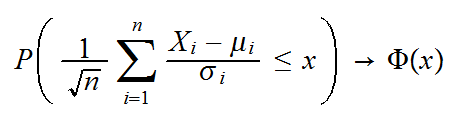
for all x, or that this standardized sum converges to a standard normal in distribution.
Note that plural "s" in the title. As with the laws of large number there are many central limit theorems, all with different conditions on
a) dependence between the Xi's
b) μi's
c) σi's
as a rough guide we have to have some combination of
a) not to strong a dependence
b) μi→μ finite
c) σi goes neither to 0 nor to ∞ to fast
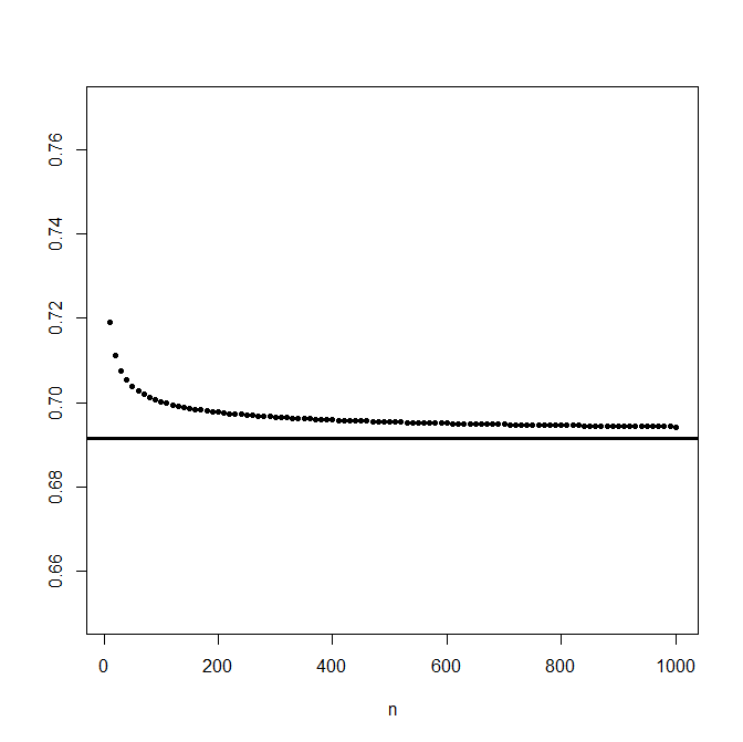
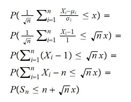
Example: Say Xi~Exp(1) independent, then we know that
EXi=1 and VarXi=1
also
Sn = X1+..Xn ~ Γ(n,1)
So
In the following graph we have these probabilities for n from 1 to 1000 for the case x=0.5, together with the clt approximation Φ(0.5)=0.69: