The Likelihood Function

One of the most important "objects" in Statistics is the likelihood function" defined as follows:

Let X=(X₁, .., X_n) be a random vector with joint pdf f(x|θ). then the likelihood function L is defined as

L(θ|x)=f(x|θ)

This must be one of the most deceivingly simple equations in math, actually it seems to be just a change in notation: L instead of f. What really matters and makes a huge difference is that in pdf we consider the x's as variables and the θ as fixed, in the likelihood function we consider the θ as the variable and the x's as fixed. Essentially we consider what happens after an experiment is done, that is what the data can tell us about the parameter.

Things simplify a bit if X₁, .., X_n is an iid sample. Then the joint density is given by

f(x|θ)=∏f(x_i|θ)

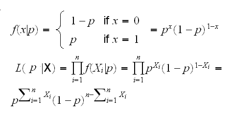
Example X₁, .., X_n~Ber(p):

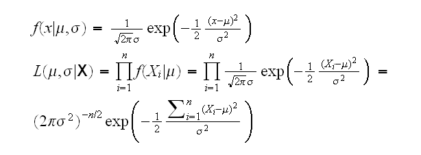
Example X₁, .., X_n~N(μ,σ):

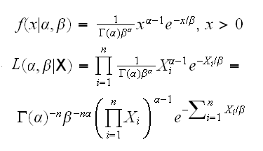
Example X₁, .., X_n~Γ(α,β):

Example An urn contains N balls. n _i of these balls have the number "i" on them, i=1,..,k and ∑n_i=N. Say we randomly select a ball from the urn, note its number and put it back. We repeat this m times. Let the rv X_i be the number of balls with the number i that were drawn, and let X=(X₁, .., X_k).

the pmf of X is given

for any x₁,..,x_k with x_i≥0 and ∑x_i=m

Now let's assume we don't know n₁,..n_k and want to estimate them. First we can make a slight change in the parameterization:

p_i=n_i/N i=1,..,k

The resulting random vector is called the multinomial rv with parameters m, p₁, .., p_k.

Note if k=2 X₁~Bin(m,p₁) and X₂~Bin(m,p₂), so the multinomial is a generalization of the binomial.

the likelihood function is given by

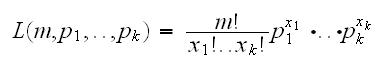
where p₁+.+.p_k=1 and x₁+..x_k=m

There is a common misconception about the likelihood function: because it is the same as the pdf (pmf) it has the same properties. This is not true because the likelihood function is a function of the parameters, not the variables.

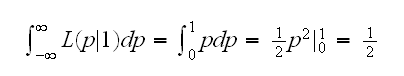
Example X~Ber(p), so f(x)=(1-p)^1-xp^x, x=0,1, 0<p<1

As a function of x with a fixed p we have f(x)≥0 for all x and f(0)+f(1)=1 but as a function of p with a fixed x, say x=1, we have

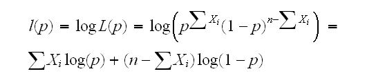
It turns out that for many problems the log of the likelihood function is more manageable entity, mainly because it turns the product into a sum:

Example X₁, .., X_n~Ber(p)

(worry about X_i=0 for all i or X_i=1 for all i yourself)

Example X₁, .., X_n~N(μ,σ):

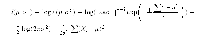
Notice that as a function of μ the log-likelihood curve of a normal is a quadratic. The coefficient in front of the quadratic term is negative, so its graph is a parabola that opens downward. Moreover, the log like-lihood is a sum of iid terms (X_i-μ)² , so an application of the central limit theorem shows that the same is true quite often even if the original distribution is not normal.

Example say X_i~Exp(λ), i=1,2,.. and the X_i are independent. Then

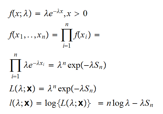
In the following 4 graphs we draw this curve for n=10, λ=1 and 4 random samples: