which rejects H0 if |T| > tα/2,n-1. So it accepts H0 if |T| ≤ tα/2,n-1 and we have the acceptance region A(μ0) = { X1, .., Xn: |T| ≤ tα/2,n-1}. Now
and so a 100(1-α)% confidence interval for μ is given by
 A(θ0)}. In other words the confidence interval is the set of all parameters for which the hypothesis test would have accepted H0.
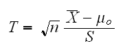
Example : Let X1, .., Xn iid N(μ,σ). Say we want to find a confidence interval for μ. To do this we first need a hypothesis test for H0: μ=μ0 vs. H1: μ ≠μ0. Of course we have the 1-sample t-test with the test statistic
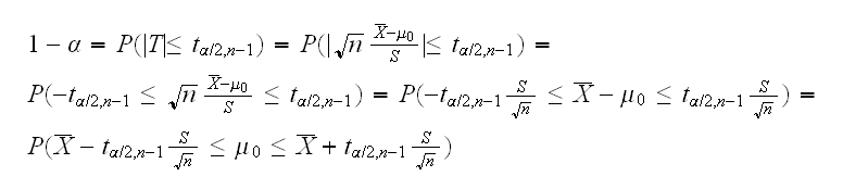
which rejects H0 if |T| > tα/2,n-1. So it accepts H0 if |T| ≤ tα/2,n-1 and we have the acceptance region A(μ0) = { X1, .., Xn: |T| ≤ tα/2,n-1}. Now
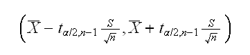
and so a 100(1-α)% confidence interval for μ is given by
Example Let's look at another example to illustrate the important point here. Let's say we have X1, .., Xn~Ber(p) and we want to find a 100(1-α)% CI for p. To do so we first need to find a test for H0:p=p0 vs Ha: p≠p0. Let's find the LRT test. Let X=∑Xi, then

binom.ex(1) draws the curve for λ(x) which shows that "λ(x) is small" is equivalent to "|X-np0| is large", and so the LRT test uses a rejection region of the form C(X)={|X-np0|>c}. What is c? We have
α=P(reject H0|p=p0)=P(|X-np0|>c)=1-P(|X-np0|≤c)=1-P(-c≤X-np0≤c)=1-P(np0-c≤X≤np0+c)
so
1-α=P(np0-c≤X≤np0+c) = pbinom(np0+c,n,p0)-pbinom(np0-c-1,n,p0)
binom.ex(2) draws the curve for pbinom(np0+c,n,p0)-pbinom(np0-c-1,n,p0) as a function of c, and finds the smallest integer c such that pbinom(np0+c,n,p0)-pbinom(np0-c-1,n,p0) ≥1-α
So for p0=0.5 and n=100 we find c=8. Therefore the test is as follows: reject the null hypothesis if |X-50|>8. This is the same as X<42 or X>58.
binom.ex(3,p0=0.5) draw the corresponding picture. It plots a dot for each possible observation X (0-n), in blue if observing this value leads to accepting the null hypothesis, in red if it means rejecting H0.
binom.ex(4,p0=0.5) draws the same graph, but now for "all" possible values of p0. This graph tells us everything about the test (for a fixed n). For example, say we wish to test H0: p=0.25 and we observe X=31, then drawing binom.ex(4,p0=0.25,X=31) shows that we should accept the null hypothesis because the intersection of the two lines is in the blue (acceptance) region..
The idea of inverting the test is now very simple: for a fixed (observed) X=x0, what values of p lead to accepting the null hypothesis? binom.ex(5,X=31) draws the same graph as before, but now finding those values of p which lead to accepting the null hypothesis.
Example : Suppose we have X1, .., Xniid Exp(β) and we want a confidence interval for β. Again we start by considering the hypothesis test
H0: β=β0 vs. H1: β≠β0.
Let's first derive the LRT for this problem. We have

In expci we draw the LRT statistic as a function of β (for A(β) and of x (for C(x)).
The expression defining the confidence interval depends on x only throughX̅. So we can write it in the form C(x) = {β: L(X̅) ≤ β ≤ U(X̅)} for some functions L and U which are determined so that the interval has probability 1-α.
Also note that the height of the curve at the left and the right confidence interval limit is the same, so
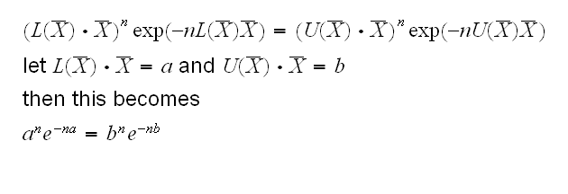
Now note that X1+..+Xn ~ Γ(n,1/β) and it is easy to show that β(X1+..+Xn) ~ Γ(n,1). So the confidence interval becomes {β: a/X̅ ≤ β ≤ b/X̅}, where a and b satisfy
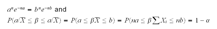
This system of nonlinear equations will of course have to be solved numerically.
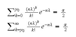
Example : Say X1, .., Xn iid P(λ). Let Y=∑Xi, than Y~Pois(nλ). Say we observe Y=y0. We have previously found a hypothesis test for H0: λ=λ0 vs. H1: λ≠λ0. It had the acceptance region A(λ0) = {qpois(α/2,nλ0)/n ≤X̅ ≤ qpois(1-α/2,nλ0)/n}. Inverting this test means solving the equations
In general this might have to be done numerically. Here, though, we can take advantage of the equation linking the Poisson and the Gamma distributions: If X~Γ(n,β) and Y~P(x/β) then P(X≤x) = P(Y≥n). Using β=2, n=y0+1, and x = 2nλ we have
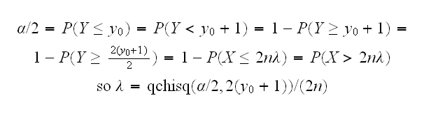
Using a similar calculation for the lower bound we find
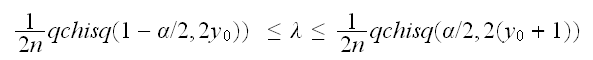
where if y0=0 we have Χ2(1-α/2,0) = 0
The routine poisci with method=1 finds this confidence interval. They are called Garwood intervals (1932)
This confidence interval has correct coverage by construction, so we don't need to worry about that as we would if our method used some approximation, say. Nevertheless, let's do a coverage study of our method. Often this has to be done with simulation, but here we can calculate it directly. Say we want to check α=0.05, n=5, λ=5.0, so nλ=25. Then from poisci we see that any value of ∑x=16 to ∑x=35 gives an interval which contains λ=5.0, so
Coverage = dpois(16,25)+dpois(17,25)+..+dpois(35,25) = 0.9552
This is done in poiscov for λ=0.001:(0.001):10 and desired values of n and α.
Notice the ragged appearance of the graph. This is typical for coverage graphs of discrete r.v, here is why: in the table we have the following: say we have one observation X from a Poisson rv. Then (if λ is small) the likely values of X are in the first column. If we observed X=0 we could find a 95% CI for λ using the method above, which gives limits L=0.000 and U=3.689, and similar for the other values of X. Now say we want to find the coverage for λ=10.3. In this case if X=5,..,17 the corresponding limits all include λ=10.3, and so the coverage is the sum of the corresponding probabilities, shown in column 4 in red, with the sum in the last row, for a coverage of 0.957. Now if we slowly raise λ, for a while it will still be X=5:17 which yield correct intervals, but the probabilities will get smaller, for a smaller (but still correct coverage). Column 5 shows the case λ=10.66.
At some point, though, the true λ will pass one of the limits, and then we get a jump in the coverage. In column 6 we have λ=10.7, and now X=5:18 yields correct intervals, and the coverage jumps up to 0.968.
| X | L | U | λ=10.3 | λ=10.66 | λ=10.67 |
| 0 | 0.000 | 3.689 | 0.000 | 0.000 | 0.000 |
| 1 | 0.025 | 5.572 | 0.000 | 0.000 | 0.000 |
| 2 | 0.242 | 7.225 | 0.002 | 0.001 | 0.001 |
| 3 | 0.619 | 8.767 | 0.006 | 0.005 | 0.005 |
| 4 | 1.090 | 10.242 | 0.016 | c0.013 | 0.013 |
| 5 | 1.623 | 11.668 | 0.032 | 0.027 | 0.027 |
| 6 | 2.202 | 13.059 | 0.056 | 0.048 | 0.048 |
| 7 | 2.814 | 14.423 | 0.082 | 0.073 | 0.073 |
| 8 | 3.454 | 15.763 | 0.106 | 0.097 | 0.097 |
| 9 | 4.115 | 17.085 | 0.121 | 0.115 | 0.115 |
| 10 | 4.795 | 18.390 | 0.125 | 0.123 | 0.122 |
| 11 | 5.491 | 19.682 | 0.117 | 0.119 | 0.119 |
| 12 | 6.201 | 20.962 | 0.100 | 0.105 | 0.106 |
| 13 | 6.922 | 22.230 | 0.079 | 0.086 | 0.087 |
| 14 | 7.654 | 23.490 | 0.058 | 0.066 | 0.066 |
| 15 | 8.395 | 24.740 | 0.040 | 0.047 | 0.047 |
| 16 | 9.145 | 25.983 | 0.026 | 0.031 | 0.031 |
| 17 | 9.903 | 27.219 | 0.016 | 0.020 | 0.020 |
| 18 | 10.668 | 28.448 | 0.009 | 0.012 | 0.012 |
| 19 | 11.439 | 29.671 | 0.005 | 0.006 | 0.007 |
| 20 | 12.217 | 30.888 | 0.002 | 0.003 | 0.003 |
| 21 | 12.999 | 32.101 | 0.001 | 0.002 | 0.002 |
| 22 | 13.787 | 33.308 | 0.000 | 0.001 | 0.001 |
| 23 | 14.580 | 34.511 | 0.000 | 0.000 | 0.000 |
| 24 | 15.377 | 35.710 | 0.000 | 0.000 | 0.000 |
| 0.957 | 0.956 | 0.968 |