 θ
θ Θ
Θ
Example : A census of all the students at the Colegio 10 years ago showed a mean GPA of 2.75. In our survey of 150 students we find today a mean GPA of 2.53. How much (if at all) has the GPA changed?
The problem of course is that the sample mean GPA depends on the sample, if we repeated our survey tomorrow with a different sample of 150 students, their mean GPA will not again be 2.53. But how far away from 2.53 might it be? Could it actually be higher than 2.75?
One way to answer such questions is to find an interval estimate rather than a point estimate.
Θ. Then (L(X), U(X)) is a 100(1-α) confidence interval for θ iff
P(L(X)≤θ≤U(X))=1-α θΘ
Example say X1, .., Xn~N(μ,σ), then a 100(1-α)% confidence interval for the population mean is given by
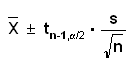
Here tn,α is the 1-α critical value of a t distribution with n degrees of freedom, that is
tn,α=qt(1-α,n)
Notice that the interval is given in the form point estimate ± error, which is quite often true in Statistics, although not always.
Example confidence interval for the mean (cont): Now

Example (GPA cont.)
and so our 90% confidence interval is (2.53-0.088, 2.53+0.088) = (2.442, 2.618)
What does that mean: a 90% confidence interval for the mean is (2.442, 2.618)? The interpretation is this: suppose that over the next year statisticians (and other people using statistics) all over the world compute 100,000 90% confidence intervals, many for the mean, others maybe for medians or standard deviations or ..., than about 90% or about 90,000 of those intervals will actually contain the parameter that is supposed to be estimated, the other 10,000 or so will not.
It is tempting to interpret the confidence interval as follows: having found our 90% confidence interval of (2.442, 2.618), we are now 90% sure that the true mean GPA (the one for all the students at the Colegio) is somewhere between 2.442 and 2.618. This, though, is incorrect. Remember that in the frequentist interpretation of probability a parameter is a fixed number. After having calculated L(X) and U(X), so are these. So interpreting a confidence interval as a probability would be like saying: the probability of
2.3 < 4.5 < 5.1
is 90%! Now clearly this is nonsense. It is just as much nonsense (not so obvious) to say that the probability of
2.442 < μ< 2.618
is 90%.
The main property of confidence intervals is their coverage, that is just the equation above.
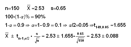
Example say X1, .., Xn~Ber(p), then by the CLT
so we have a candidate for a 100(1-α)% CI. But this is based on the CLT, so there is a question how large n needs to be for this to work. Let's check the coverage of this method:
First of all it will depend on n and p. To illustrate, let's find the coverage for the case n=20, p=0.43. Now first we can find all the intervals for n=20:
x
x/n
L
U
0
0.00
0.000
0.000
1
0.05
-0.046
0.146
2
0.10
-0.031
0.231
3
0.15
-0.006
0.306
4
0.20
0.025
0.375
5
0.25
0.060
0.440
6
0.30
0.099
0.501
7
0.35
0.141
0.559
8
0.40
0.185
0.615
9
0.45
0.232
0.668
10
0.50
0.281
0.719
11
0.55
0.332
0.768
12
0.60
0.385
0.815
13
0.65
0.441
0.859
14
0.70
0.499
0.901
15
0.75
0.560
0.940
16
0.80
0.625
0.975
17
0.85
0.694
1.006
18
0.90
0.769
1.031
19
0.95
0.854
1.046
20
1.00
1.000
1.000
Notice that for x=5 to x=12 we have intervals that contain p=0.43, so the true coverage is
P(X=5)PP(X=6)+..+P(X=12) = 0.932
where X~Bin(20,0.43).
Now we repeat this for p=0.01 to 0.99 in steps of 0.01 and draw the true coverage:
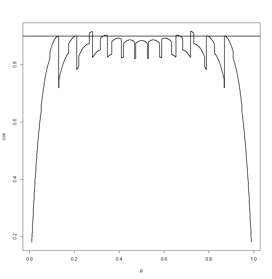
and we see that this method really does not work very well. And yet this is the standard method in every textbook, and taught to every student of Statistics!
Well, maybe the problem is that n=20 is not large enough. Here is the graph for n=200:
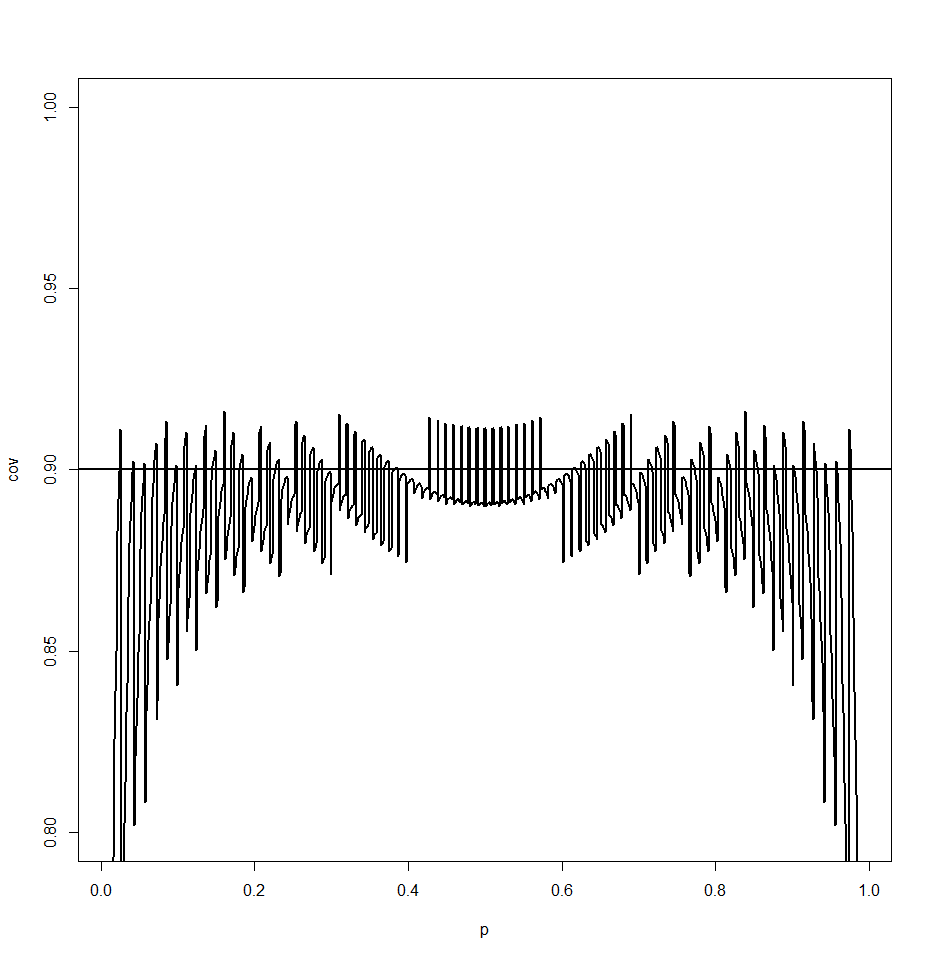
Better, but still not very good.
Θ. Then (L(x), U(x)) is a 100(1-α)% credible interval for θ iff
P(L(x)≤θ≤U(x)|X1=x1, .., Xn=xn)=1-α
Notice now the data appears in the conditional part, so this is a probability based on the posterior distribution of θ|X1=x1, .., Xn=xn
Example say X1, .., Xn~N(μ,σ)
T keep things simple we will assume that σ is known, so we just need a prior on μ. Let's say μ~N(μ0,τ) Then

so the posterior distribution of μ|X=x is again a normal.
How can we get a credible interval from this? The definition above does not determine a unique interval, essentially we have one equation for two unknowns, so we need an additional condition. Here are some standard solutions:
a) equal tail probability interval: choose L and U such that
P(L(x)<θ|X1=x1, .., Xn=xn)=α/2 and P(θ>U(x)|X1=x1, .., Xn=xn)=1-α/2
Example (GPA cont.) First we need to choose σ, μ0 and τ Let's use σ=0.65, μ0=3.0 and τ=1.0, then
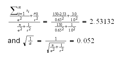
and we find L(x)=qnorm(0.025,2.53132,0.052)=2.429 and U(x)=qnorm(0.975,2.53132,0.052)=2.633
b) highest posterior density interval. In addition to the first equation we also have
fθ(L(x)|X1=x1, .., Xn=xn)=fθ(U(x)|X1=x1, .., Xn=xn)
In our case this yields the same interval as in a) because the nromal density is symmetric around the mean.
c) quantiles from simulated data. If we can sample from the posterior distribution we can use these. Say Y1,..,Y1000
are 1000 simulated observations from μ|X=x, then (Y[25], Y[975]) is a 90% credible interval.
The main property of credible intervals is just the equation that defines them.
Example say X1, .., Xn~Ber(p), and let's use as a prior on p the U[0,1]. Then
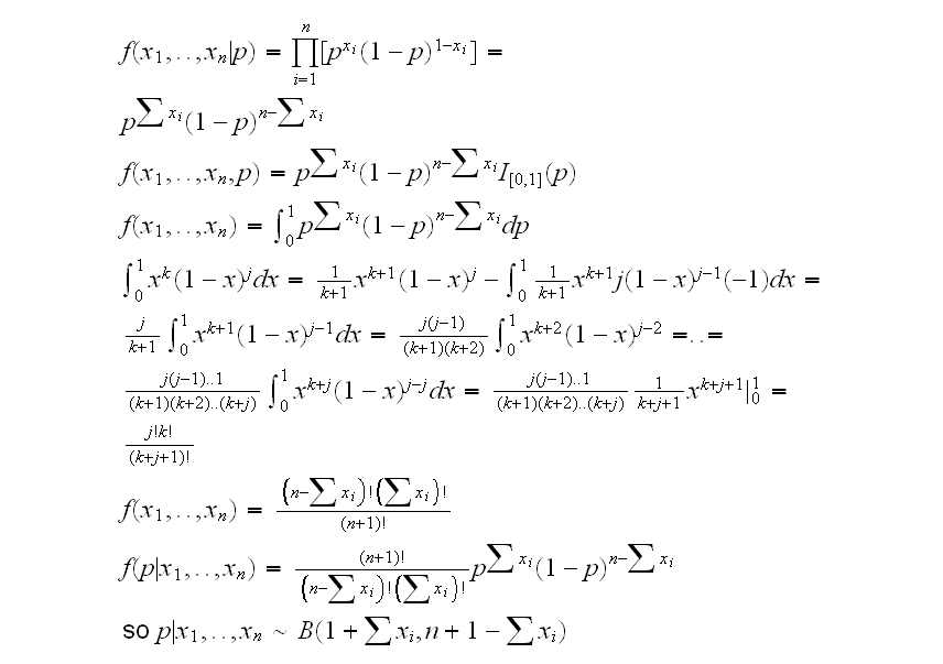
Now if we use the equal tail probabilities method we find L(x)=qbeta(0.025,1+sum(x), n+1-sum(x)) and U(x)=qbeta(0.975,sum(x),n+1-sum(x))
In cibernoulli(2) we generate B=1000 p~U[0,1], then generate sum.x=∑x~Ber(p) and finally find the percentage of intervals (L(sum.x),U(sum.x)) that contain their respective p.
Example say X1, .., Xn~N(μ,σ) and we are interested in estimating μ and σ simultaneously. So we want to find a region A(x) 2such that
P((μ,σ)A(X))=1-α
We already know thatX̅ and s are good point estimators of μ and σ. Morover it can be shown thatX̅ s, so
s, so
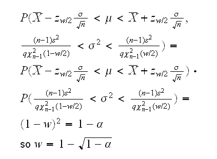
confreg.norm shows that this indeed has the right level α. What does this region look like? confreg.norm(2) draws the region.