 Θ0
Θ0Example: A new textbook for Introductory Statistics has just been released. It has some inovative ideas and might be an improvement over the current textbook. Rather than just switching, we decide to be good scientists and base our decision on facts. So we set aside one section of the course next semester and use the new textbook in this section.
Based on what information are we going to make our decisions? We could look at the percentage of students who pass the class, at the scores in the partial exams, the overall grade distribution etc. Let's say we decide to focus on the score in the final exam, mainly because we know that the mean score over the last 5 years with the current textbook has been 73 points.
Now of course if the students in this section have a mean score less than 73, we clearly won't change. But what if it is a little bit higher, say 75 points? Could a 2 points difference be just due to random chance, or is it "proof" that the new textbook is better? If not 75, how about 77? 80? How much better does the mean score have to be for us to decide that the next textbook is better? A hypothesis test can tell us!
H0: θΘ0
where θ is a parameter (vector) and Θ0 is a region in the parameter space Θ
Example X~Ber(p), Θ=[0,1], Θ0={0.5}, so we are testing whether p=0.5
Example X~N(μ,σ), Θ= x(0,∞), Θ0=(100,∞)x(0,∞), so we are testing whether μ>100
In addition to the null hypothesis we also write down the alternative hypotheses Ha, usually (but not always) the complement of Θ0. So a hypothesis test makes a choice between H0 and Ha.
A complete hypothesis test should have all of the following parts:
1) Type I error probability α
2) Null hypothesis H0
3) Alternative hypothesis Ha
4) Test statistic
5) Rejection region
6) Conclusion
Example: Over the last five years the average score in the final exam of a course was 73 points. This semester a class with 27 students used a new textbook, and the mean score in the final was 78.1 points with a standard deviation of 7.1.
Question: did the class using the new text book do (statistically significantly) better?
For this specific example the hypotheses are of course
H0: μ = 73 (no difference between textbooks) vs Ha: μ > 73 (new textbook is better than the old one)
How should we decide to whether to accept or reject H0? Clearly if the mean score using the new textbook is much higher than the mean score before we would reject it. So it makes sense to look at
X̅-μ
Now even if the new textbook is the same as the old one, X̅ might still be a little bit bigger than 73 due to random chance. After all, even in the past half the sections had a mean score over 73! If we want to be reasonably sure that it is really better we should require that
X̅ - μ > c
where c is a constant choosen such that P(X̅ - μ > c) is small if the null hypothesis is true.
Let's say we decide we want
P(X̅ - μ > c) = α
for some small α, say 0.05 or 0.01.
Notice it says if the null hypothesis is true. So here we consider what would happen if the new textbook is NOT better than the old one, that is the scores on the final exam are still going to be just like they were with the old textbook. Because we are considering the sample mean X̅ we can (hopefully) use the central limit theorem and we therefore know that
X̅ ~N(μ,σ)
where μ=73. We do not know the population standard deviation σ, but we have the sample standard deviation s=7.1. Therefore
T = √n(X̅-μ)/s ~ tn-1
Of course
X̅ - μ > c
is equivalent to
T = √n(X̅-μ)/s > c'
How do we find c'? Well: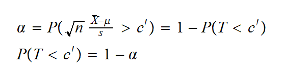
so c' is the 1-α percentile of a t distribution with n-1 degrees of freedom. Here n=27, 1-α=1-0.05=0.95, so
t26,0.95=1.706
http://www.tutor-homework.com/statistics_tables/statistics_tables.html#t
in our case we find
T = √n(X̅-μ)/s = √27(78.1-73)/7.1 = 3.732 > 1.706, so we reject the null hypothesis, it appears that the mean score in the final is really higher.
When we carry out a hypothesis test in the end we always face one of the following situations:
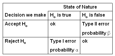
So when we do a hypothesis test there are two possible mistakes: falsely rejecting the H0 or falsely accepting H0. These are called the tyoe I and type II errors. Each mistake happens with some probability, called α and β. Here the similarity ends, though: we specify α, but we have so far said nothing about β.
In some ways you can think of hypothesis testing as a procedure designed to control α!
How do you choose α? This in practise is a very difficult question. What you need to consider is the consequences of the type I and the type II errors. As discussed here hypothesis testing is a procedure designed to help make decisions. Well, false decisions have consequences!
Example: In our textbook example we have
Type I error: Reject H0 although H0 is true
H0: μ=73 (mean score on final is the same as before, new textbook is not better than old one)
This is the truth, but we don't know this, based on our experiment and the hypothesis test we reject H0, that is now we think the textbook is better
Consequences?
• We will change textbooks for everybody
• New students will not be able to buy used books, previous students will not be able to sell their books
• Professors have to rewrite their material, prontuarios etc.
• Professors will not consider other new textbooks that might really be better
• but scores will not go up, all of this is for nothing
Type II error: Fail to reject H0 although H0 is false
H0: μ=73 (mean score on final is the same as before, new textbook is not better than old one)
This is false, but we don't know this, based on our experiment and the hypothesis test we fail to reject H0, that is now we think the textbook is not better
Consequences?
• We will not change to the new textbook
• scores will not go up, but they would have if we had changed
• more students would have passed the course, got an A etc., but now they won't
• Professors will consider other new textbooks, but those might really be worse than the one we just rejected.
Is there any of these consequences we should try very hard to avoid? If is is one of those under the Type I error, choose a small α, say 0.01 or even 0.0001. If it is one of the consequences of the type II error, allow a larger α, say 0.1 or 0.2.
Many fields such as psychology, biology etc. have developed standards over the years. The most common one is α = 0.05, and we will use this if nothing else is said.
In real live a frequentist hypothesis test is usually done by computing the p-value, that is the probability to observe the data or something even more extreme given that the null hypothesis is true
Example (above)
p = P(mean score on final exam > 78.1 | μ = 73) = P(T>3.732) = 0.000468
Then the decision is made as follows:
| p< α | p> α |
| reject H0 | fail to reject H0 |
The advantage of the p value approach is that in addition to the decision on whether or not to reject the null hypothesis it also gives us some idea on how close a decision it was. If p=0.035 < α=0.05 it was a close decision, if p=0.0001<α=0.05 it was not.
The correct interpretation of the p-value is one of the differences between the Fisher and the Neyman-Pearson theories of hypothesis testing. In the case of Neyman-Pearson it is simply a 1-1 transformation of the test statistic, used to simplify the decision of whether to reject the null hypothesis. It would not be correct to interpret the p-value as evidence against the null, as it would be in a Fisherian test.
The p-value depends on the observed sample, which is a random variable, so it in turn is a random variable. What is its distribution?
Example say X~N(μ,1) and we want to test H0: μ=0 vs Ha: μ>0. We use the rejection region {X>cv} where cv=zα, the critical value from a standard normal distribution. Now let Y~N(μ,1) independent of X, assume we observe X=x and denote the p-value by p(x), then
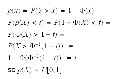
so if the null hypothesis is true the distribution of the p-value is uniform [0,1]. This turns out to be true in general.
To begin with, if we wanted to test the hypothesis H0: θ=θ0 we would need to start with a prior that puts some probability on the point {θ0}, otherwise the hypothesis will always be rejected. If we do that we can simply compute P(H0 is true | data), and if this probability is smaller than some threshhold (similar to the type I error) we reject the null hypothesis.
Instead of the probability P(H0 is true | data) we often compute the Bayes factor, given as follows: say X1, .., Xn~f(x|θ) and θ~g, then the posterior density is
g(θ|x) proportional to L(θ)g(θ)
The belief about H0 before the experiment is descibed by the prior odds ratio P(θΘ0)/P(θΘ1), and belief about H0 after the experiment is descibed by the posterior odds ratio P(θΘ0|x)/P(θΘ1|x). The Bayes factor is then the ratio of the posterior to the prior odds ratios (a ratio of ratios)