In a hypothesis test the type I error probability α is defined by
α=P(reject H0|H0 is true)
and is chosen by the analyst at the beginning of the test. On the other hand the type II error probability β is defined by
P(accept H0| H0 is false)
Example say we have X1, .., Xn~Ber(p) and for some reason we want to test
H0: p=0.5 vs Ha: p=0.6.
Now X̅ is the mle of p and a large value of X̅ indicates that the null hypothesis is wrong, so we might use a test with the rejection region {X̅>cv} for some critical value cv. Say Y~Bin(n,0.5). Then
α = P(X̅>cv|p=0.5) =
1-P(∑X≤n·cv|p=0.5) =
1-P(Y≤n·cv)
1-α = P(Y≤n·cv)
n·cv=qY(1-α)
cv=qY(1-α)/n
where qY(1-α) ist the (1-α)100 percentile of a binomial distribution (n,0.5).
Now say Z~Bin(n,0.6), then
β = P(X̅≤cv|p=0.6) = P(∑X≤n·cv|p=0.6) = P(Z≤n·cv) = P(Z≤n·qY(1-α)/n)
As a numerical example say α=0.05 and n=100, then cv=0.58 and β=0.3774
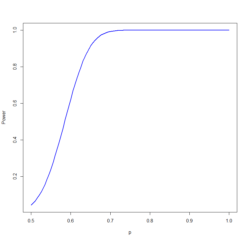
Example say we have X1, .., Xn~Ber(p) and now we want to test H0: p=0.5 vs Ha: p>0.5.
It starts out exactly the same as before, and again we find
cv=qY(1-α)/n
but when we want to find β we have a problem, we don't know what the p is. What we can do is find β as a function of p:
β(p) = P(X̅≤cv|p) = P(∑X≤n·cv|p)
In real life we usually calculate the power of the test, defined by
Pow(p)=1-β(p)
It has two advantages:
1) it gives the probability of corrrectly rejecting a false null hypothesis
2) Pow(p0)=α
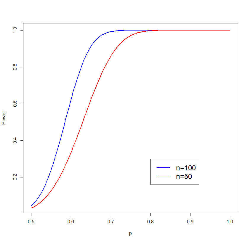
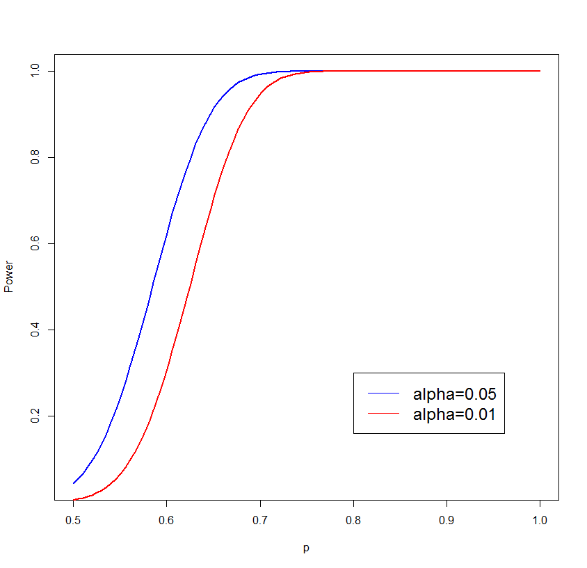
Here is the power curve for n=100, α=0.05
To compare, here is the powercurve if n=50
and if α=0.01:
Example say we have X1, .., Xn~N(μ,σ), σ known, and now we want to test
H0: μ=μ0 vs Ha: μ≠μ0
Again X̅ is the mle, and
Z=√n(X̅-μ0)/σ ~N(0,1)
so a test might use the rejection region {|Z|>cv}:
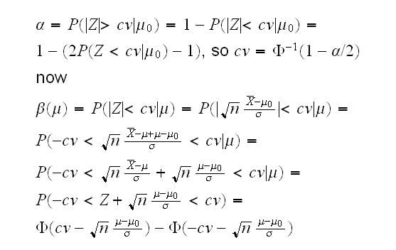
Here is what this looks like for n = 99, μ0 = 0, σ = 1 and α = 0.05:
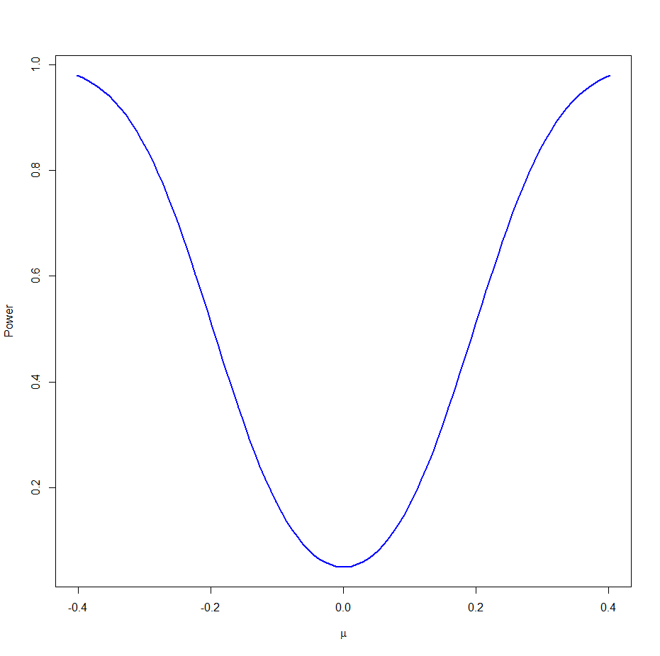
Example Again we have X1, .., Xn~N(μ,σ), σ known, and now we want to test H0: μ=μ0 vs Ha: μ≠μ0 , but this time we will use the median M as an estimator of μ. Again a reasonable rejection region is {|M-μ|>cv}. The problem is, what is the distribution of M? It can be found, but we won't worry about that here. If we have it, though, we can again find the power curve. The next graph draws the power curves of the median (in red) together with the power of the test based on the sample mean (in blue).
as we can see the power of the test based on the mean is higher, and that is the reason why this test is preferred.
Example say X1,..,Xn~Ber(p), and we want to test H0: p=p0 vs. Ha:p>p0. As above a reasonable test can be based on {X̅>cv}, which is equivalent to {∑xi≥k} for some integer k. Say for example n=10, p0=0.5 and α=0.1. Then
P(∑Xi≥10)= 0.00097
P(∑Xi≥9)= 0.0107
P(∑Xi≥8)= 0.0547
P(∑Xi≥7)= 0.1719
so for k=8 P(reject H0|H0 is true)<α and for k=7 P(reject H0|H0 is true)>α. Because of the discreteness of the random variable it is not actually possible to find a cv such that P(reject H0|H0 is true)=α. In this case we use min{k: P(reject H0|H0 is true)<α} or k=8.
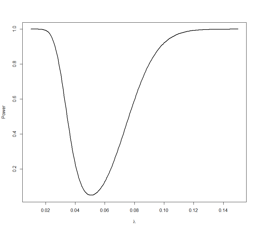
Example: Say we have the following sample:
1 1 2 2 2 2 5 6 7 7 11 11 12 13 14 21 24 28 29 32 34 39 44 83 103
say from the experiment is is reasonable to believe that this is a sample from an exponential distribution with rate λ. We suspect that λ=1/20. So we want to test
H0: λ=1/20 vs. Ha λ≠1/20.
Let's start by finding the maximum likelihood estimator. We have previously seen that if Sn=X1+..Xn the log-likelihood function is given by
l(λ) = n log λ - λSn
so
l'(λ) = n/λ - Sn = 0
mle = n/Sn = 1/X̅ = 25/533 = 0.0469
so if H0 is true we would expect 1/X̅ to be close to 1/20, or equivalently X̅ close to 20, or equivalently S25 close to 25*20=500
but S25 is the sum of independent exponential random variables and therefore if H0 λ=1/20 is true we have
S25 ~ Gamma(25, 20)
It seems reasonable to reject H0 if either S25 << 500 or if S25>>500, so we have a rejection region of
{S25 <c1 or S25>c2}
Of course our test needs to have a significance level of α, so we need
P(S25 <c1 or S25>c2|λ=1/20)=α
but that is just one equation for two unkowns. In general we need another one. Often what is done is to split this in two equal parts:
P(S25 <c1|λ=1/20)=α/2 and P(S25>c2|λ=1/20)=α/2
so c1 is the α/2 quantile of a Γ(25,20) distribution. If we use α=0.05 we can find
c1=323.6 and c2=714.2
we have S25 = 533, so we fail to reject the null hypothesis.
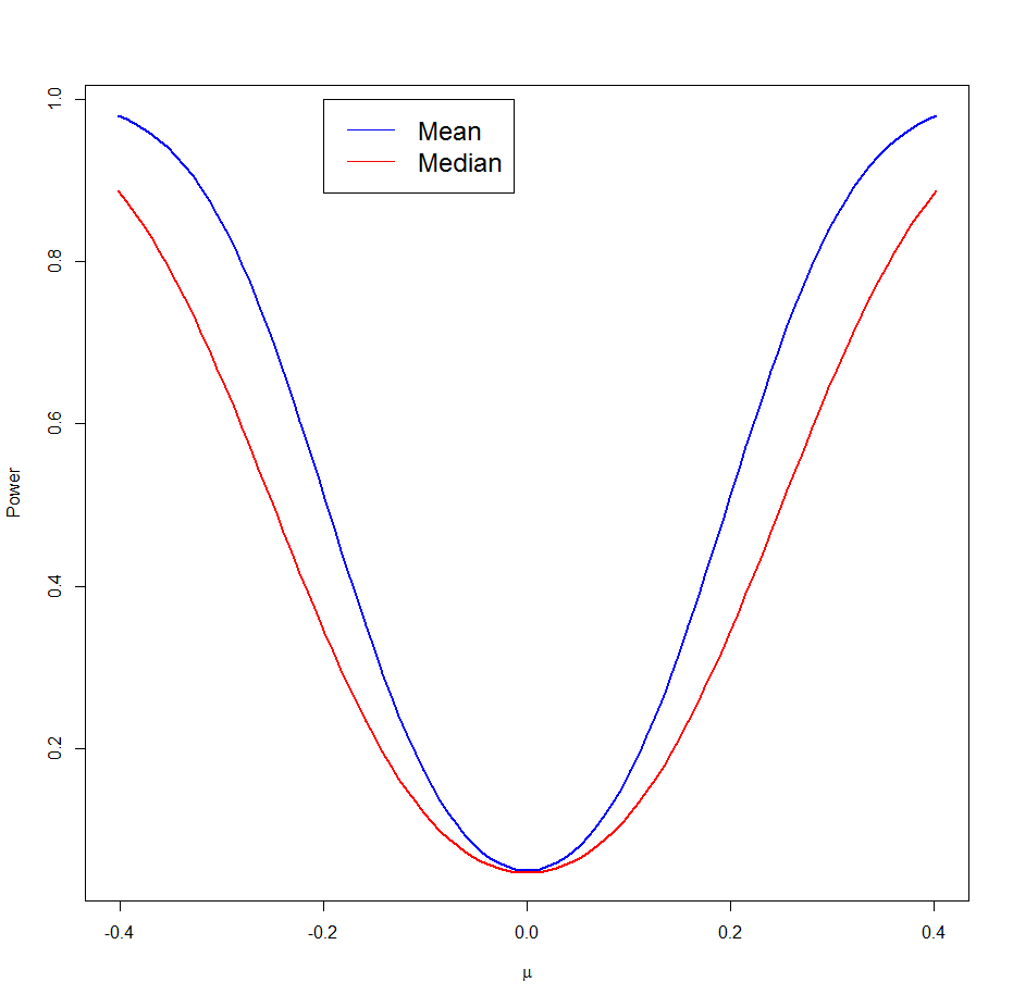
What is the power of this test? Well, let Y~Γ(25,λ), then
Power(λ) = P(reject H0 |true rate is λ) = P(Y<323.6 or Y>714.2)
and is drawn here: