
which has a chisquare distribtuin with 3 (4-1) degrees of freedom (-1 because of ∑pi=1)
For Mendels' data we find E = (312.75, 104.25, 104.25, 34.75), so χ2=0.47 and therefore p-value=1-pchisq(0.47,3)=0.92
Often in Statistics we assume that the data was generated by a specific distribution, for example the normal. If we are not sure that such an assumption is justified we would like to test for this.
Example : Say we have X1, .., Xn iid F, and we wish to test H0: F=N(0,1)
First notice that here the alternative hypothesis is H0: F ≠N(0,1), or even simply left out. Either way it is a HUGE set, made up of all possible distributions other than N(0,1). This makes assessing the power of a test very difficult.
Example : Another famous data set in statistics is the number of deaths from horsekicks in the Prussian army from 1875-1894, in horsekicks. It has been hypothesized that this data follows a Poisson distribution. Let's carry out a hypothesis test for this.
First of a Poisson distribution has a parameter, λ. Clearly even if the assumption of a Poisson distribution is correct it will be correct only for some values of λ. The mle of λ is the sample mean, here 9.8, and in some sense if any Poisson distribution fits the data, the Poisson with mean 9.8 should. So we will test specifically F = Pois(9.8)
The chisquare goodness-of-fit test is a large-sample test, it has the sassumption that none of the expected numbers be to small. For example we find E(0) = 20*P(X=0)= 20*dpois(0,9.8) = 0.0. We deal with this by combining some categories. With this we find the following table:
| Number of Horsekicks | 0-6 | 7-9 | 10-12 | 13 or more | Total |
| Observed | 6 | 4 | 5 | 5 | 20 |
| Expected | 2.8 | 6.8 | 6.5 | 3.9 | 20 |
and we find c2 = 5.32.
Under the null hypothesis the c2 statistic has a c2 distribution with m-k-1 degrees of freedom, where m is the number of classes and k is the number of parameters estimated from the data. So here we have m-k-1 = 4-1-1 = 2 d.f, and we find a p-value of 0.07, indicting that the data might well come from a Poisson distribution.
In the binning we have used, some E are a bit small. We could of course bin even further, but then we also lose even more information. Instead we can use simulation to find the p value. The routine horsekicks.fun carries out the calculations.
Example : Say we have a data set and we want to test whether is comes from a normal distribution. In order to use the c2 test we first need to bin the data. There are two basic strategies:
a) Use equal size bins (with the exception of the first and the last)
b) Use adaptive bins chosen so that each bin has roughly the same number of observations.
The routine normal.chisq carries out both versions.
Testing for normality is a very important problem, although because of simulation not quite as important today as it used to be. There are a number of test available for this problem, most of them much better (that is with higher power) than the chisquare test. Look for example for the Shapiro-Wilks test and the Anderson-Darling test.
A very good way to assess the distribution of a sample (such as normality) is to draw a graph specifically designed for this purpose, the probability plot. It plots the sample quantiles vs. the quantiles of the hypothesized distribution. If the data follows that distribution the resulting plot should be linear. In R we have the routine qqplot and for the normal distribution especially we have qqnorm. qqline adds a least squares fitted line to help with reading the graph. One important use of this graph is that it also provides some insight on what the true distribution looks like. qq.ill does some examples.
Kolmogorov-Smirnov Test
Say we have X1, .., Xn which are continuous and independent r.v. and we wish to test H0: Xi~F for all i. Above we talked about graphs that give us some idea whether the data really comes from a certain distribution. Now let's use the empirical distribution function. If the null hypothesis is true, than the empirical cdf should be close to the true one, that is the "distance" between the two curves should be small.
How can we define this "distance"? in mathematics there are a number of possible definitions:
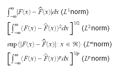
We are going to consider the L∞ norm here, so we have the test statistic
D = max{|F(x)-Fhat(x)|:x 
 }.
}.
This is called the Kolmogorov-Smirnov statistic.
At first glance it appears that computing D is hard: it requires finding a maximum of a function which is not differentiable. But inspection of the graphs (and a little calculation) shows that the maximum has to occur at one of the jump points, which in turn happen at the observations. So all we need to do is find F(Xi)-Fhat(Xi) for all i.
Next we need the null distribution, that is the distribution of D if the null hypothesis is true. The full derivation is rather lengthy and won't be done here, but see for example J.D Gibbons, Nonparametric Statistical Inference. The main result is that if F is continuous and X~F, then F(X)~U[0,1], and therefore D does not depend on F, it is called a distribution-free statistic. It's distribution can be found by simply assumimg that F is U[0,1].
The method is implemented in R in the routine ks.test where x is the data set and y specifies the null hypothesis, For example y="pnorm" tests for the normal distribution. Parameters can be given as well. For example ks.test(x,"pnorm",5,2) tests whether X~N(5,2).
Note that this implementation does not allow us to estimate parameters from the data. Versions of this test which allow such estimation for some of the standard distributions are known, but not part of R. We can of course use simulation to implement such tests.
It is generally recognized that the Kolmogorov-Smirnov test is much better than the Chisquare test.
For our general discussion this test is interesting because it does not derive from any specific principle such as the likelihood principle. It si simply an idea (let's compare the cdf under H0 with the empirical cdf) and a lot of heavy probability theory. Such methods are quite common in Statistics.