 = T(X1, ..,Xn) is called unbiased for θ if
 Definition
An estimator = T(X1, ..,Xn) is called unbiased for θ if
E =θ
B( ) = E -θ
is called the bias of the estimator T
Example: say X1, ..,Xn are iid with mean μ and standard deviation σ. Then
EX̅ = E[(1/n)∑Xi] = (1/n)∑E[Xi] = (1/n)∑μ = (1/n)*nμ = μ
so X̅ is an uniased estimator of μ
How about the variance σ2? Here we will use as an estimator the sample variance
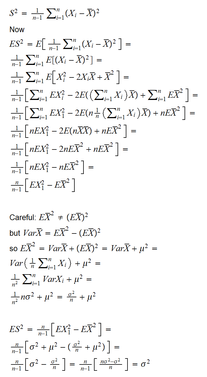
and this of course explains why we use "n-1" instead of "n".
How about the standard deviation σ? Unfortunately
E√S2 ≠ √ES2
(actually, a famous inequality called Jensen's inequality says E√S2 ≤ √ES2)
so S = √S2 is NOT an unbiased estimator of the standard devation s. In fact, in this generality nothing more can be said. Howerver, if we also assume that the Xi come from a normal distribution it can be shown (Holzman 1950) that
E[cnS]=σ
where
cn = {Γ[(n-1)/2][(n-1)/2)]1/2}/Γ(n/2)
Surprised that the Gamma function shows up here? Remember that if Xi,..,Xn is iid Normal, S2 has a chisquared distribution and the chisquare is a special case of thr Gamma distribution.
Example: say X1, ..,Xn are iid U[0,θ]. Find an unbiased estimator of θ.
we have Xi<θ for all i, so max{Xi}<θ as well. In fact we would expect the largest of the Xi to be close to θ. So let's try as an extimator T=max{Xi}
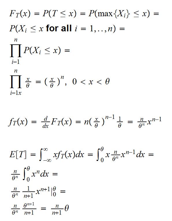
so T is not an unbiased estimator of θ, but of course it is easy to make it so, just use (n+1)/nθ!
Let X = X1, ..,Xn be a sample from a distribution with pmf(pdf) f(x|θ1,..,θk).
Definition
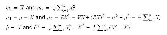
the ith sample moment is defined by
mi = (Xi1+..+Xin)/n
Analogously define the ith population moment by
μi = EXi
Of course μi is a function of the θ1,..,θk. So we can find estimators of θ1,..,θk by solving the system of k equations in k unknowns
mi=μi i=1,..,k
Example: say X1, ..,Xn are iid U[0,θ]
we have
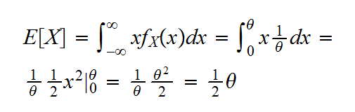
so we get
m1 = μ1 = θ/2
or = 2m1 = 2X̅
Example : say X1, ..,Xn are iid N(μ,σ).
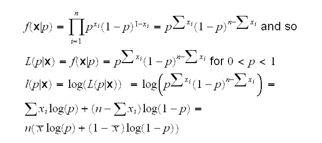
The idea here is this: the likelihood function gives the likelihood (not the probability!) of a value of the parameter given the observed data, so why not choose the value that "matches" (gives the greatest likelihood) to the observed data.
Example: say X1, ..,Xn are iid Ber(p). First notice that a function f has an extremal point at x iff log(f) does as well because
d/dx{log(f(x))}=f'(x)/f(x)=0 iff f'(x)=0
Now
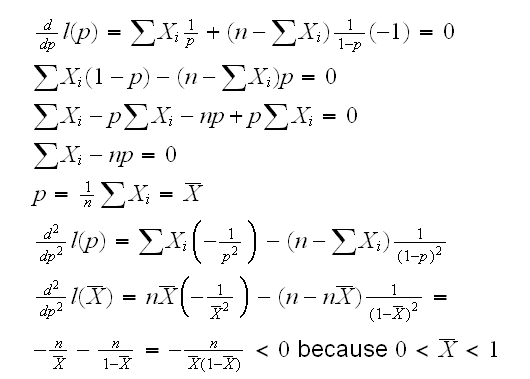
Here we verified that the extrema is really a maxima. Recall that we previously said that the log-likelihood of the normal distribution as a function of μ is a quadratic opening downward, and that because of the central limit theorem the log-likelihood function of many distributions approaches that of a normal. For this reason the log-likelihood function (almost) always has a maximum at the mle. There are exceptions, though:
Example: say X1, ..,Xn are iid U[0,θ], θ>0. Then
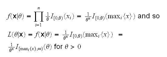
Now L(θ|x) is 0 on (0,max(xi)), at max(xi) it jumps to 1/(max(xi))n and then monotonically decreases as θ gets bigger, so the maximum is obtained at θ=max(xi), therefore the mle is max(xi)
Here is an example: say n=10 and max{xi}=1.55, then the likelihood curve looks like this
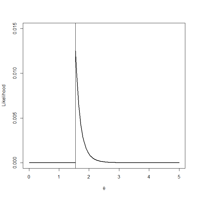
and it has its maximum at 1.55
Notice that here log f is of no use because f(x)=0 for values of x close to the point were the maximum is obtained.
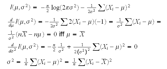
Example X1, .., Xn~N(μ,σ):
Example say X has a multinomial distribution with parameters p1,..,pk (we assume m is known), then if we simply find the derivatives of the log-likelihood we find
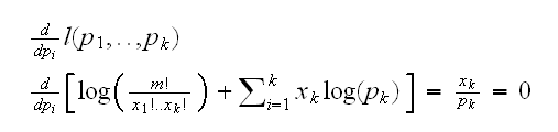
and this system has no solution. The problem is that we are ignoring the condition p1+..+pk=1. So we really have the problem
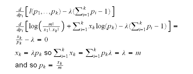
Minimize l(p1,..,pk) given p1+..+pk=1
One way to do this is with the method of Lagrange multipliers: minimize
l(p1,..,pk)-λ(p1+..+pk-1):
Maximum likelihood estimators have a number of nice properties. One of them is their invariance under transformations. That is if is the mle of θ, then g() is the mle of g(θ)
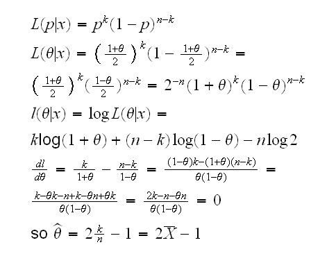
Example say X1, .., Xn~Ber(p) so we know that the mle isX̅. Say we are interested in θ=p-q=p-(1-p)=2p-1, the difference in proportions. Therefore 2X̅-1 is the mle of θ.
Let's see whether we can verify that. First if θ=2p-1 we have p=(1+θ)/2 and so
Example say X1, .., Xn~N(μ,σ) so we know that the mle of σ2 is S2 . But then the mle of σ is s.
Definition
Let X=(X1,..,Xn) be a random sample from some pmf (pdf) f(.,θ). Then the quantity
is called the Fisher information number of the sample.
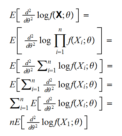
If the sample is identitically distributied things simplify:
We said before that often the log-likelihood the log-likelihood function of many distributions approaches that of a normal. We can now make this statement precise:
Theorem Let X1, .., Xn be iid f(x|θ). Let denote the mle of θ. Under some regularity conditions on f we have
√n[-θ]→N(0,√-v)
where v is the Fisher information number
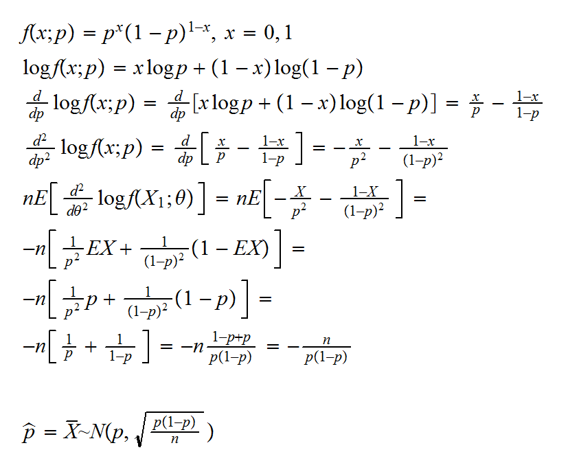
Example say X1, .., Xn are iid Ber(p) and we want to estimate p. We saw above that the mle is given by X̅ .
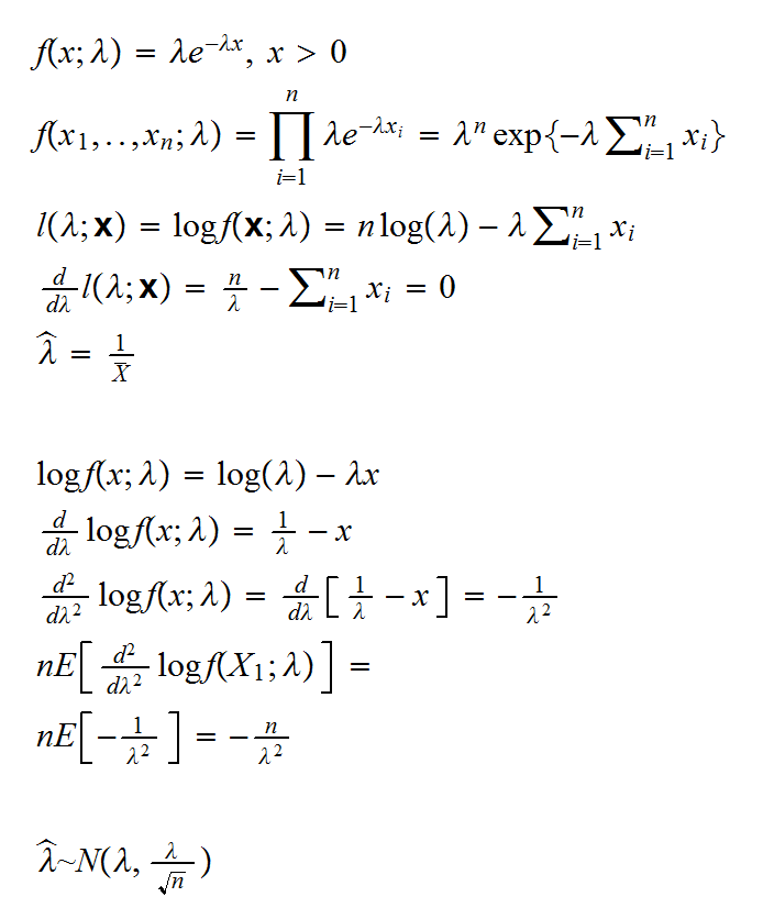
Example say Xi~Exp(λ), i=1,2,.. and the Xi are independent. Then we saw before that if Sn=(X1+..+Xn)
l(λ;x) = nlog(λ)-λSn .
Now
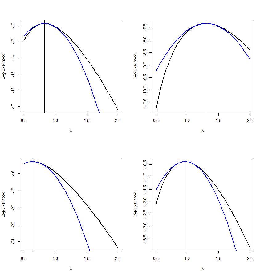
here are 4 examples. n=10, λ=1. The true log-likelihood curve is in black and the parabola from the normal approximation is in blue.
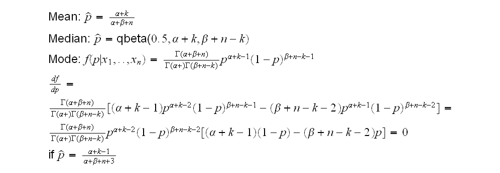
We have already seen how to use a Bayesian approach to do finding point estimators, namely using the mean of the posterior distribution. Of course one could also use the median or any other measure of central tendency. A popular choice for example is the mode of the posterior distribution.
Example Let's say we have X1, .., Xn~Ber(p) and p~Beta(α,β), then we already know that
p|x1,..xn~Beta(α+∑xi,n-∑xi+β)
and so we can estimate p as follows:
Example: A switch board keeps track of the number of phone calls they receive per hour during the day:
1 5 4 4 3 1 5 5 5 6 7 5 4 4 4 2 4 7 0 3 4 9 4 2
Let's say they believe that the number of calls has a Poisson distribution with rate λ.
a) find the maximum likelihood estimator of the rate λ
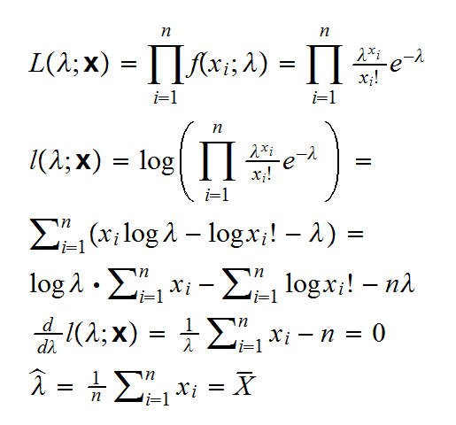
and we find X̅ = 4.08
b) Find the Bayes estimator for λ as the median of the posterior distribution . Use as a prior π(λ)=1/λ, λ>0
This is of course an improper prior because ∫π(λ)dλ=∞
Now
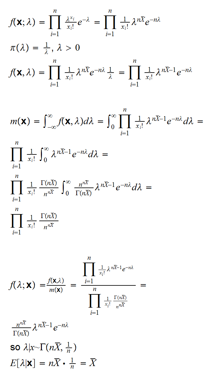
and we get the same answer!