Let's revisit some of the examples we discussed earlier, and analyse them using the bootstrap:
Example In a survey of 1000 likely voters 523 said they will vote for party A, the other 477 for party B. Find a 95% CI for the lead of one party over the other. Done in lead.boot(), compare to diffprop()
Example Recall the pet ownership and survival data:
| Patient Status |
Owns a Pet |
Does not Own a Pet |
| Alive |
50 |
28 |
| Dead |
3 |
11 |
Question: is there a statistically significant association between Ownership and Survival?
First we need a "measure of association", that is a number we can calculate from the data that tells us something about the relationship (or lack thereof) between our variables. Previously we used the chisquare statistic, so let's use it again. Only now we don't need the chisquare approximation, we can just study the distribution of the chisquare values for the bootstrap sample. In pet.boot we take bootstrap samples of the "owns" and of "survives" independently, calculate the corresponding chisquare statistics and repeat that B times. Finally we find the percentage of bootstrap runs larger than the observed chisquare, which is essentially the p-value of our test.
Example the effect of the mother's cocain use on the length of the newborn. In cocain.boot we use the bootstrap to find 95% confidence intervals for the means and medians of the lengths.
Example Consider the dataset hubble. Check hubble.boot() and comapre to hubble.est()
Example Consider Gregor Mendl's pea experiment. Check mendel.boot()
Example (from "An Introduction to the Bootstrap" by Bradley Efron and Robert Tibshirani)
The data is the thicknesses in millimeters of 485 Mexican
stamps printed in 1872-1874, from the 1872 Hidalgo issue. It is thought that the stamps from this issue are a "mixture" of different type of paper, of different thicknesses. Can we determinse from the data how many different types of paper were used?
As a first look at the data let's draw several histograms, with different bins. This is done in stamps$f(). It seems there are at least two and possibly as many as 6 or 7 "peaks" or "modes".
Here we are using the histogram as a "density estimator", that is we visualize the "top" of the histogram as a density. In stamps$f(2) we draw just that "top".
The main problem with this is that the true density is continuous but the histogram is not smooth. Instead we should use a "nonparametric density estmator" A popular choice is a kernel density estimator:
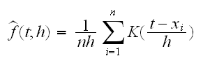
where h is called the bandwidth (equivalent to the binwidth of histograms) and K is called the kernel function. A popular choice for K is the density of a standard normal rv. In stamps$f(3) we draw four different curves for different values of h. As we can see, the smaller h gets the more ragged the curve is.
It is clear that the number of modes depends on the choice of h. It is possible to show that the number of modes is a non-increasing function of h.
Let's say we want to test H0: number of modes=1 vs. Ha: number of modes>1 Because the number of modes is non-increasing there exists an h1 such that the density estimator has one mode for h<h1 and two or more mode for h>h1. Playing around with stamps$f(4,h=..) we can see that h1~0.0068.
Is there a way to calculate the number of modes for a given h? here is one:
• calculate yi=fhat(ti;h) on a grid t 1,..tk
• calculate zi=yi-1-yi and not that at a mode z will change from positive to negative.
• # of modes = ∑I[zi>0 and zi+1<0]
In stamps$f(5,want.mode=..) we "automate the process to find the largest h which yields want.mode modes. It uses a very simple "bisection algorithm":
• start with h=0.007, which we know has just one mode
• reduce h by 0.001 until we have (at least) want. mode modes
• set low =h, high=h+0.001 (which has to include the desired h), set h=(low+high)/2 . If at h we have want. mode modes h is small enough, so we set low=h, otherwise high=h
• continuoue until |high-low|<10-7
So, how we can test H0: number of modes=1 vs. Ha: number of modes>1? Here it is:
• draw B bootstrap samples if size n from fhat(.,h1)
• for each find h1star, the smallest h for which this bootstrap sample has just 1 mode
• approximate p-value of test is #{h1star>h1}/B
Notice we don't actually need h1star, we just need to check if h1star>h1, which is the case if fhatxtar(.,h1) has at least two modes.
Note that we are not drawing bootstrap samples from "stamps" but from a density, fhat. This type of bootstrap is called a smooth bootstrap.
How do we draw from fhat? Let y1star,..,ynstar be a bootstrap sample from the data, and set
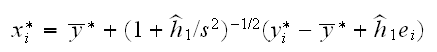
where s2 is the variance of the data and εi are standard normal rv's. The term (1+h1star/s2) insures that the bootstrap sample has the same variance as the data, which turns out to be a good idea.
Finally we can test for 2 modes vs more than 2 modes etc, in a similar fassion. The results are shown here:
| # of modes |
hm |
p-value |
| 1 |
0.0068 |
0.00 |
| 2 |
0.0032 |
0.29 |
| 3 |
0.0030 |
0.06 |
| 4 |
0.0029 |
0.00 |
| 5 |
0.0027 |
0.00 |
| 6 |
0.0025 |
0.00 |
| 7 |
0.0015 |
0.46 |
| 8 |
0.0014 |
0.17 |
| 9 |
0.0011 |
0.17 |
So there are certainly more than one mode, with a chance for as many 7.