for example if we observe X=0.45 a 95% CI for a is (0.032, 4.620)
X1, .., Xn iid F with f(x|a)=axa-1, x>0, a>0 (or simply X~Beta(a,1))
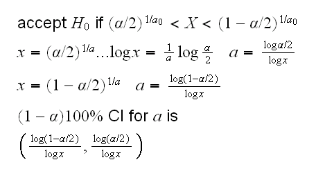
and we want to find a (1-α)100% condifence interval for a.Let's again first consider the case n=1. Previously we had the following hypothesis test for H0:a=a0 vs Ha:a≠a0: reject the null hypothesis if
X<(α/2)1/a0 or X>(1-α/2)1/a0
therefore we
for example if we observe X=0.45 a 95% CI for a is (0.032, 4.620)
This is illustrated here:
Here we split α 50-50 on the left and the the right. Is this optimal? Let's put λα on the left and (1-λ)α on the right for some 0≤λ≤1. Then
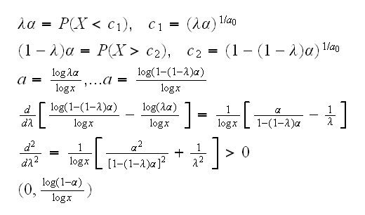
and now if we observe X=0.45 a 95% CI for a is (0, 3.75)
Note that these intervals always start at 0, which might not be a good idea for some experiments.
How about the case n=2?
We have qbeta2(α/2,a)=x which is equivalent to pbeta2(x,a)=α/2, and we need to solve this for a. Again this needs to be done numerically:
invbeta2 <-
function (x, alpha=0.05)
{
x=sum(x)
pbeta2=function(x,a) {integrate(dbeta2,0,x,a=a)$value}
low=0
repeat {
low=low+1
flow=pbeta2(x,low)
print(c(low,flow))
if(flow<1-alpha/2) break
}
high=low
low=low-1
repeat {
mid=(low+high)/2
fmid=pbeta2(x,mid)
print(c(mid,fmid))
if(abs(fmid-(1-alpha/2))<0.001) break
if(fmid>(1-alpha/2)) low=mid
else high=mid
}
L=mid
low=0
repeat {
low=low+1
flow=pbeta2(x,low)
print(c(low,flow))
if(flow<alpha/2) break
}
high=low
low=low-1
repeat {
mid=(low+high)/2
fmid=pbeta2(x,mid)
print(c(mid,fmid))
if(abs(fmid-alpha/2)<0.001) break
if(fmid>alpha/2) low=mid
else high=mid
}
H=mid
c(L,H)/2
}
For example, say we observe (x,y) = (0.31, 0.59) note that (x+y)/2 = 0.45, same as above with n=1. Then we find a 95% CI for a to be (0.039, 1.53)
Previously we also used simulation to estimate pbeta2(x,a) If we could not calculate it numerically we could use this as well, but clearly we are going to get routines that take take rather a long time to run.
And then n large:
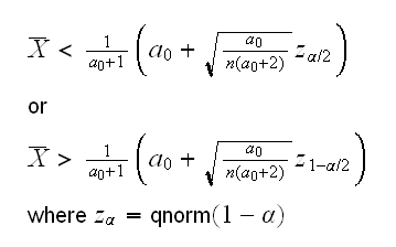
so the acceptance region of the test is
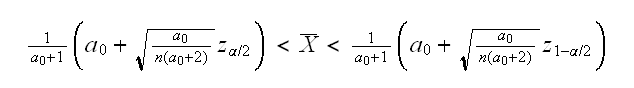
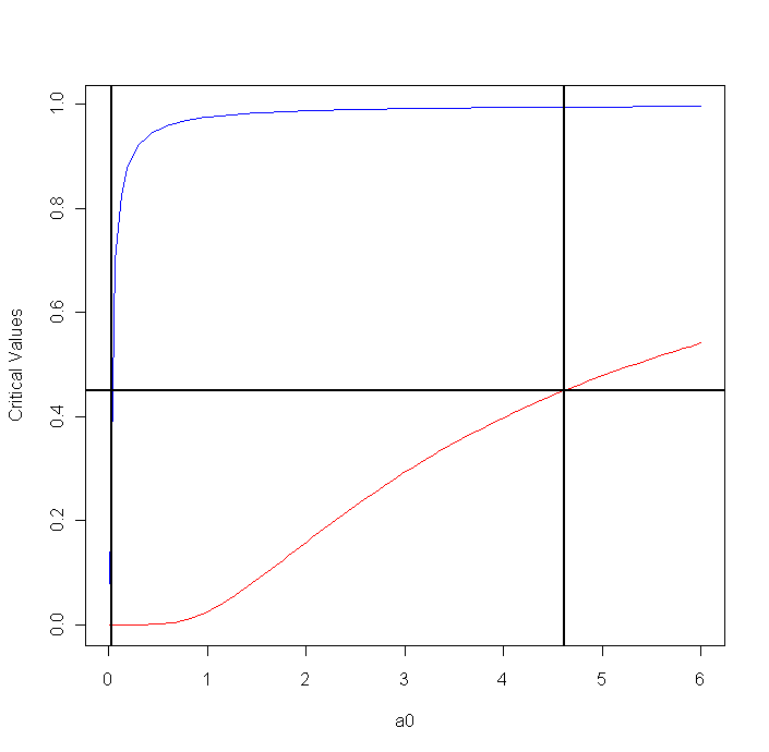
to get a confidence interval we need to "invert the test". This means solving the double-inequality in the acceptance region for a (which now replaces a0). The next graph shows the left and the right side of the double-inequality as a function of a, (blue=α/2, red=1-α/2, n=50,X̅=0.4)
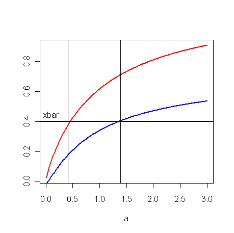
and we get an interval (0.48, 1.45)
Formally we need to solve the equation beta3.ex(1) does the calculations.
How about the mle? This one is easy: Bayesian Interval Which Interval is Better?
First of frequentist confidence intervals and Bayesian credible intervals can not really be compared directly. We will just compare the two confidence intervals.
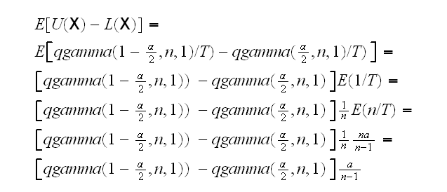
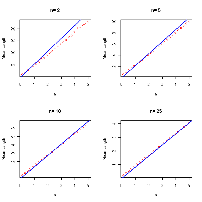
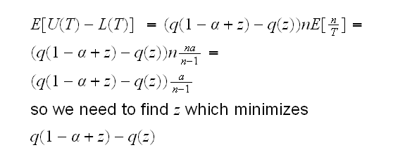
First we need to check that the two methods yield proper confidence intervals, that is that they have coverage. So if we calculate a 90% interval it really contains the true parameter 90% of the time. This is true for the LRT interval by construction because we could find the exact distribution of the LRT statistic and invert the interval analytically. The other test is a large sample test and needs to be checked via simulation. Here are some results (red=MM, blue=LRT) How can we choose between the two? We need a measure of performance for a confidence interval. Again we can consider the mean length of the interval E[U(X)-L(X)]. In the case of the MM method this will need to be found via simulation. As for the LRT method, we have Above we used the fact that aT has distribution that does not depend on the parameter a. We then found the interval by dividing the error probability α equally on the left and the right. But is that the best option? If we are interested in shortest-length intervals, can we find the intervals that are optimal? That is can we find L(T) and U(T) such that
minimize E[U(T)-L(T)] subject to P(L(T)<a<U(T))=1-α
Let's set q(z)=qgamma(z,n,1) and let's consider intervals of the form L(T)=q(z1)/T and U(T)=q(1-z2)/T. Clearly we need z1+z2=α , so we have z2=1-α+z1 or we just write
L(T)=q(z)/T and U(T)=q(1-α+z)/T
This has length How much better are these intervals? Here are the mean lengths (for a=1)
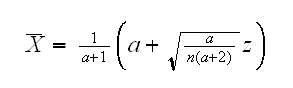
for z=zα/2 and z=z1-α/2. Let x=X̅, then
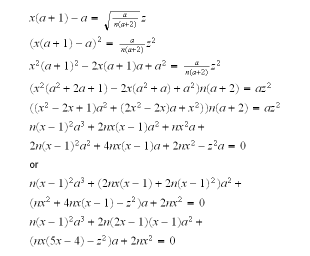
so now we have a cubic equation, which we can solve. In R this is done by the routine cuberoots. Of course there are generally three roots, but one of them is negative and the other two are our solutions. Note that zα/22=qnorm(1-α/2)2=qnorm(α/2)2=z1-α/22 , so we only need to solve one equation.
beta3.ex(2) does the work.
Previously we saw that if we use a prior Exp(1) we get a posterior distribution a|x~Γ(n+1,1/(T+1)) using this we can find the equal-tail probability interval by solving
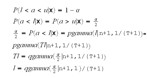
which is (almost) the same as the confidence interval based on the LRT test.
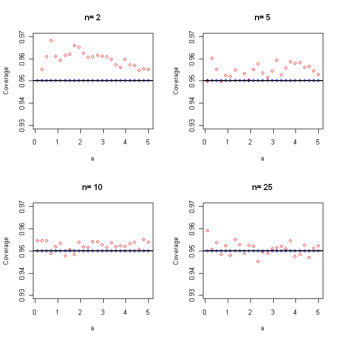
so we see that the MM method has some over-coverage for small n. Over-coverage is acceptable but not really desirable because it generally mean larger intervals.
Here is a graph of the mean lengths:
This can not be done analytically, and so again we need to resort to a numerical solution. In beta3.ex(3) i use a simple "grid-search" algorithm. It turns out that assigning a smaller part of α to the left side leads to shorter intervals.
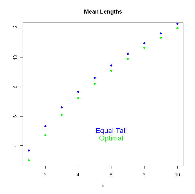
For example if n=2 (and a=1) the mean length of the equal-tail intervals is 5.33 but for the "optimal" length intervals it is 4.72, an improvement of about 10%