 .
.
Say X1, .., Xn iid F with f(x|a)=axa-1, x>0, a>0 (or simply X~Beta(a,1))
say we want to test H0:a=a0 vs Ha:a≠a0.
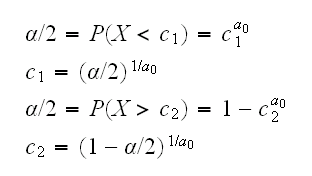
let's first consider the case n=1. We already know that EX=a/(a+1), so X~a/(a+1) or a~X/(1-X). So a test could be based on the rejection region X/(1-X)<c1 or X/(1-X)>c2. But the function x/(1-x) is monotonically increasing, so this rejection region is equivalent to one with X<c1 or X>c2, and so
.
For example if we wish to test a0=0.5 we reject the null hypothesis if X<0.000625 or X>0.950625.
How about n=2, say X and Y? Again we might try to use the fact that E[(X+Y)]/2 = a/(1+a) But eventually we would need to find the density of X+Y:
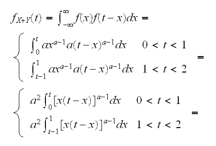
and these intergals don't exist. What can we do? One idea is to find the integral numerically:
dbeta2 <-
function (x,a=1)
{
f=function(x,t) {(x*(t-x))^(a-1)}
y=0*x
for(i in 1:length(x)) {
if(x[i]<1) y[i]=integrate(f,0,x[i],t=x[i])$value
else y[i]=integrate(f,x[i]-1,1,t=x[i])$value
}
a^2*y
}
pbeta2 <-
function(x,a=1)
{
y=x
for(i in 1:length(x)) y[i]=integrate(dbeta2,0,x[i],a=a)$value
y
}
qbeta2 <-
function (p,a=1)
{
pbeta2=function(x) {integrate(dbeta2,0,x,a=a)$value}
low=0
high=2
repeat {
mid=(low+high)/2
fmid=pbeta2(mid)
if(abs(fmid-p)<0.001) break
if(fmid<p) low=mid
else high=mid
}
mid
}
and qbeta2(0.025,1/2)=0.03 qbeta(0.975,1/2)=1.6
so we reject the null hypothesis if (X+Y)/2<0.015 or (X+Y)/2>0.8
Alternatively we can use simulation to find the null distribution:
xy=matrix(rbeta(20000,0.5,1),10000,2)
z=apply(xy,1,sum)
quantile(z,c(0.025,0.975))
5% 95%
0.0335 1.586
and so again we reject the null hypothesis if (X+Y)/2<0.015 or (X+Y)/2>0.8
This of course works equally well for n=3, 4, ... whereas the numerical solution gets much harder quickly.
How about n large? From the CLT we know that
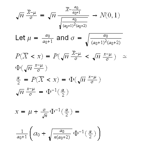
similarly for 1-α/2. So we have the following test for H0:a=a0 vs Ha:a≠a0: reject H0 ifX̅<x orX̅>y where
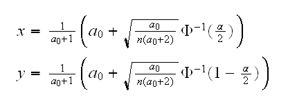
One-sided tests: above we tested H0:a=a0 vs Ha:a≠a0. Often we want to test instead alternatives of the form Ha:a<a0 or Ha:a>a0. In that case choose the appropriate rejection region, with α instead of α/2
p-value: if we want to quote the p-value of this test we calculate it as follows: say we observedX̅=t in our experiment. The p-value is the probability of repeating the experiment and observing a value of the test statistic as "unlikely" (given the null hypothesis) as that seen in the original experiment. Say we observed t>a0 and let Ybar be the sample mean of the new experiment, then
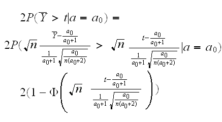
the "2" is because we do a two-sided test.
How about the likelihood ratio test? We have
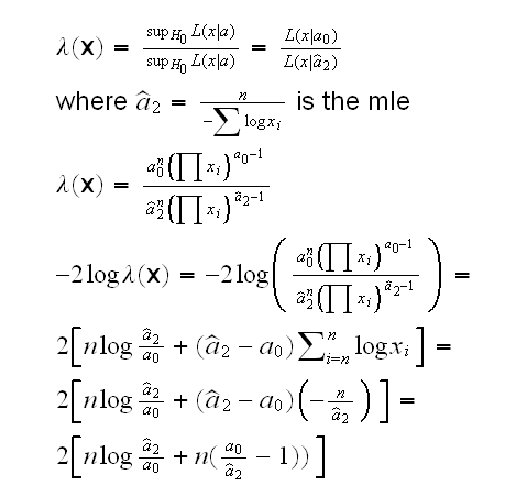
and we reject H0 if -2logλ(x)>qchisq(1-α,1)
One problem with both these methods is that they are large sample methods, they rely on the CLT. Can we derive a method that also works for small samples? The basic idea of the LRT is to reject the null hypothesis if λ(x) is small, which is the same as (-2)logλ(x) is large. Now consider this:
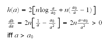
so h is decreasing on (0,a0) and increasing on (a0,∞), or so h is large for small or large values of a.
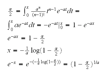
Now a2hat=n/T, and so "a2hat is small or large" is equivalent to "T is small or large". If H0 is true T~Γ(n,1/a0) and if we α/2 on the left and the right we find
α/2=P(T<x)=pgamma(x,n,a0)
x=qgamma(1-α/2,n,a0)
Similarly α/2=P(T>y) y=qgamma(1-α/2,n,a0) and so we reject H0 if
T<qgamma(α/2,n,a0) or T>qgamma(1-α/2,n,a0)
Note
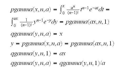
so we reject H0 if
a0T<qgamma(α/2,n,1) or a0T>qgamma(1-α/2,n,1)
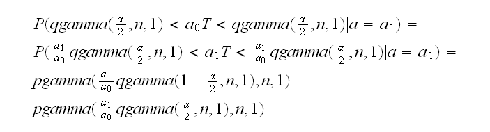
One-sided tests: Say we want to test Ha:a<a0 Then we have the rejection region a0T<qgamma(α,n,1)
p-value: p=2P(T*>t|a=a0) =2(1-pgamma(t,n,a0)) if t>a0 or p=2P(T*<t|a=a0) =2pgamma(t,n,a0) if t<a0
How about a Bayesian method? Let's use again the prior Exp(1), then we know a|x~Γ(n+1,T+1) A test could be designed as follows: reject H0 if a0<qgamma(α/2,n+1,T+1) or a0>qgamma(1-α/2,n+1,T+1). But from the above we know that
a0<qgamma(α/2,n+1,T+1)=qgamma(α/2,n+1,1)/(T+1)
iff
a0(T+1)<qgamma(α/2,n+1,1)
and we see that this is essentially the same as the test based on the mle. (except with n+1 instead of n and T+1 instead of T)
Let's go back to the two tests based on the sample mean and the likelihood ratio. Which of these is best? That depends on the power of the test. First we have
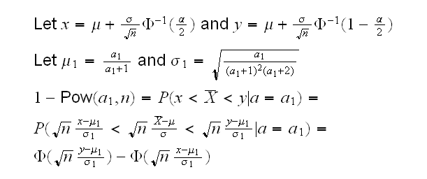
and then
beta1.ex(5) draws the power curves.
Of course the Wald type test only works for large samples. A difficult question is how large n needs to be. Simulation can help to decide that.
We also have two tests for the case n=1. How do they relate to each other? For the test based on the likelihood ratio statistic we reject H0 if
T<qgamma(α/2,n,a0) or T>qgamma(1-α/2,n,a0)
but now T=-logX so
-logX<qgamma(α/2,n,a0) or -logX >qgamma(1-α/2,n,a0)
or
X<exp{-qgamma(1-α/2,n,a0) } or X> exp{-qgamma(α/2,n,a0) }
for the direct test we reject H0 if
X<(α/2)1/a0 or X>(1-α/2)1/a0
Let's draw this regions as a function of a0:
cvn1 <-
function (alpha=0.05)
{
a0=seq(0.1,10,length=100)
cv1=(alpha/2)^(1/a0)
cv2=(1-alpha/2)^(1/a0)
cv1a=exp(-qgamma(1-alpha/2,1,a0))
cv2a=exp(-qgamma(alpha/2,1,a0))
plot(a0,cv1,type="l",col="red",ylim=c(0,max(cv2,cv2a)))
lines(a0,cv2,col="red")
lines(a0,cv2,col="blue")
lines(a0,cv2a,col="blue")
cbind(a0,cv1,cv1a,cv2,cv2a)
}
and we see they are the same! Here is why: qgamma(qgamma(alpha/2,1,a0) is the solution to the equation
How about n=2? This is much trickier because one test is based on x+y, the other one on log(x)+log(y) Here is a little simulation:
cvn2 <-
function (m=1000)
{
r=matrix(0,m,2)
for(i in 1:m) {
xy=rbeta(2,1/2,1)
if(sum(xy)<0.03125 | sum(xy)>1.593) r[i,1]=1
if(-sum(log(xy))<0.484 | -sum(log(xy))>11.14) r[i,2]=1
if(r[i,1]!=r[i,2]) return(xy)
}
NULL
}
which shows that sometime one test rejects H0 while the other does not.
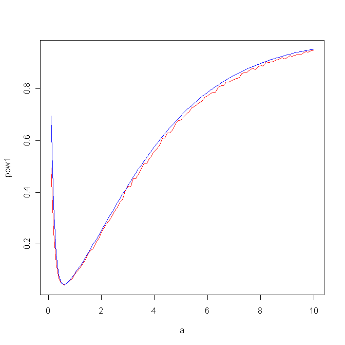
so then which is better? We do have a formula for the power of the likelihood ratio test, the other one needs to be done via simulation. Here is the result for a0=0.5:
powern2 <-
function (a0=1/2,m=100)
{
xy=matrix(rbeta(20000,a0,1),10000,2)
z=apply(xy,1,sum)
cv=quantile(z,c(0.025,0.975))
a=seq(0.1,10,length=m)
pow1=rep(0,m)
for(i in 1:m) {
xy=matrix(rbeta(20000,a[i],1),10000,2)
z=apply(xy,1,sum)
z1=z[z<cv[1]]
z2=z[z>cv[2]]
pow1[i]=length(c(z1,z2))/10000
}
pow2=1-(pgamma(a/a0*qgamma(0.975,2,1),2,1)-pgamma(a/a0*qgamma(0.025,2,1),2,1))
plot(a,pow1,type="l",col="red")
lines(a,pow2,col="blue")
}