So the posterior distribution of p|Y=y is again a Beta, but now with parameters y+1 and n-y+1.
"The probability of rain tomorrow is 40%"
This seemingly simple and obvious statement is something that you have heard many times, but have you ever considered what it really means? Trying to define the meaning of probability has turned out to be quite difficult. From its beginnings in the 17th century Probability Theory had a hard time doing that. Every time someone proposed a definition someone else shortly found that this definition lead to some contradiction!
For probability theory this only ended when Kolmogorov in the 1930s decided to not say what a probability is but how it behaves, by stating his famous three axioms.
Unfortunately this simple way out does not work for Statistics, we have to relate our theories to real live experiments and so we have to say exactly what we mean by a statement like the above. From the beginning of Statistics there have been two main definitions:
Frequentist: as long run percentage of repeated experiments
(historically on .. it rains on 40% of the days)
Bayesian: as a degree of believe
( it is my personal experience that at this time of the year it rains about 4 out of 10 days)
Both of these definitions have their strength and their weaknesses. The main problem with the frequentist definition is its limited applicability. What sense does it make to imagine a "long-run" repetition of an experiment when the experiment is one that can only done once, such as the experiment "what is the probability that i will have a car accident tomorrow?". Notice this is me, and not anyone else, and it is tomorrow, and not any other day of my life!
The main problem with the Bayesian definition is its subjectiveness. It is my personal opinion that the chance of rain tomorrow is 40%, it does not have to be yours, you can have your own!
In the Bayesian approach θ is considered a quantity whose variation can be described by a probability distribution (called a prior distribution), which is a subjective distribution describing the experimenters belief and which is formulated before the data is seen. A sample is then taken from a population indexed by θ and the prior distribution is updated with this new information. The updated distribution is called the posterior distribution. This updating is done using Bayes' formula, hence the name Bayesian Statistics.
Let's denote the prior distribution by π(θ) and the sampling distribution by f(x|θ), then the joint pdf (pmf) of X and θ is given by
f(x,θ)=f(x|θ)π(θ)
the marginal of the distribution of X is
m(x)=∫ f(x|θ)π(θ)dθ
and finally the posterior distribution is the conditional distribution of θ given the sample x and is given by
π(θ|x) = f(x|θ)π(θ)/m(x)
We can write this also in terms of the the likelihood function:
π(θ|x1,..,xn) = L(θ|x1,..,xn)π(θ)/m(x)
Example: You want to see whether it is really true that coins come up heads and tails with probability 1/2. You take a coin from your pocket and flip it 10 times. It comes up heads 3 times. As a frequentist we would now use the sample mean as an estimate of the true probability of heads, p and find p̂ = 0.3.
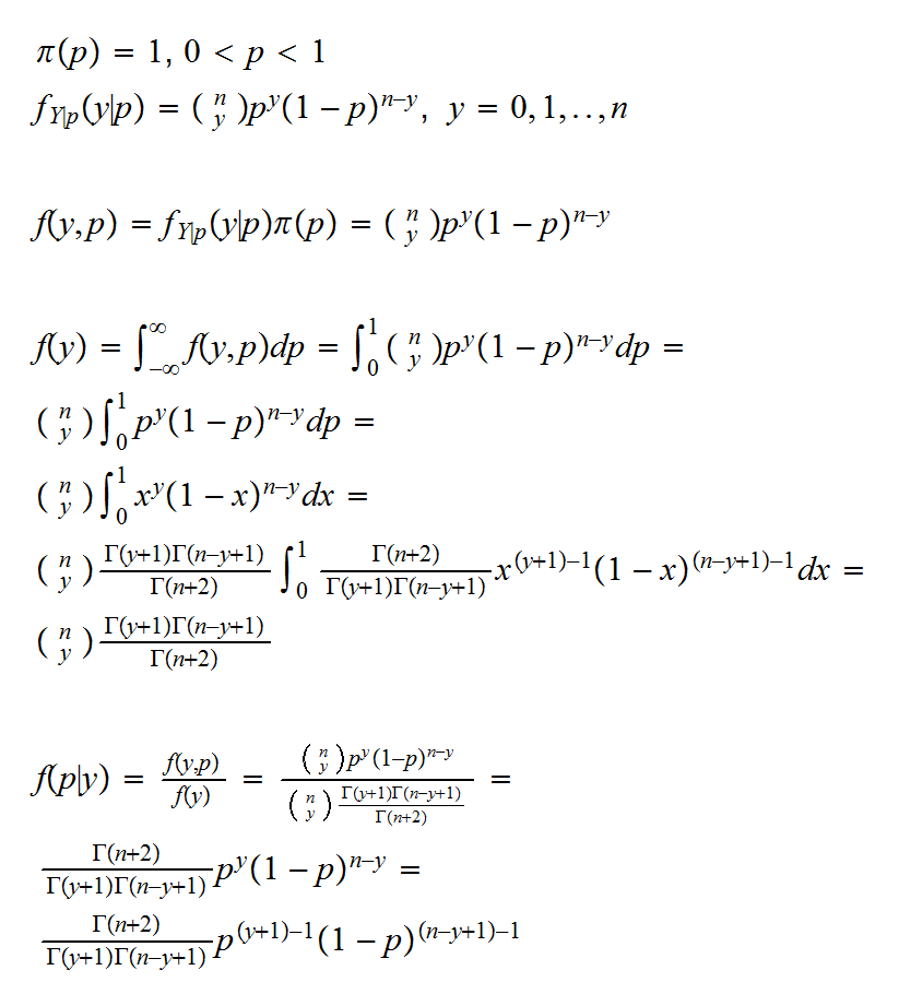
A Bayesian analysis would proceed as follows: let X1, .., Xn be iid Ber(p). Then Y= X1+..+ Xn is Bin(n,p). Now we need a prior on p. Of course p is a probability, so it has values on [0,1]. One distribution on [0,1] we know is the Beta, so we will use a Beta(α,β) as our prior. Remember, this is a perfectly subjective choice, and anybody can use their own. The joint distribution on Y and p is given by
So the posterior distribution of p|Y=y is again a Beta, but now with parameters y+1 and n-y+1.
Of course we still need to "extract" some information about the parameter p from the posterior distribution. Once the sampling distribution and the prior are chosen, the posterior distribution is fixed (even though it may not be easy or even possible to find it analytically) but how we proceed now is completely open and there are in general many choices. If we want to estimate p a natural estimator is the mean of the posterior distribution, given here by
p̂B = (y+1)/(n+2) = 4/11
• Should you buy a new car, or keep the old one for another year?
• Should you invest your money into the stock market or buy fixed-interest bonds?
• Should the goverment lower the taxes or instead use the taxes for direct investments?
In decision theory one starts out by choosing a loss function, that is a function that assigns a value (maybe in terms of money) to every possible action and every possible outcome.
Example You are offered the following game: you can either take $10 (let's call this action a), or you can flip a coin (action b). If the coin comes up heads you win $50, if it comes up heads you loose $10. So there are two possible actions: take the $10 or flip the coin, and three possible outcomes, you win $10, $50 or loose $10. We need a value for each combination. One obvious answer is this one:
L(a)=10, L(b,"heads")=50, L(b,"tails")=-10
But there are other possibilities. Say you are in a bar. You already had food and drinks and your tab is $27. Now you notice that you only have $8 in your pocket (and no credit card etc.) Now if you win or loose $10 it doesn't matther, either way you can't pay your bill, and it will be very embarrassing when it comes to paying. But if you win $50, you are fine. Now your loss function might be:
L(a)=0, L(b,"heads")=1000, L(b,"tails")=0
The next piece in decision theory is the decision function. The idea is this: let's carry out an experiment, and depending on the outcome of the experiment we chose an action.
• Should you invest your money into the stock market or buy fixed-interest bonds?
Let's do this: we wait until tommorrow. If the Dow Jones goes up, we invest in the stock market, otherwise in bonds.
In decision theory a decision rule is called inadmissible if there is another rule that is better no matter what the outcome of the experiment. Obviously it makes no sense to pick an inadmissible rule.
So what's the connection to Bayesian Statistics? First there are Bayesian decision rules, which combine prior knowledge with the outcome of the experiment.
• based on the movement of the Dow Jones in the last year, I have a certain probability that it will go up over the next year.
Now there is a famous theorem (the complete class theorem) that says that all admissible rules are Bayesian decision rules for some prior.
Example one of the most useful modern methods, called the Bootstrap, is a purely Frequentist method with no Bayesian theory. (Actually there is something called the Bayesian bootstrap, but it is not the same as the classical bootstrap)
Example A standard technic in regression is to study the residuals. This, though, violates the likelihood principle and is therefore not allowed unter the Bayesian paradigm. Actually, most Bayesians study the residuals anyway.