under the null hypothesis μ1=...=μk=μ and so
Example Chasnoff and others obtained several measures and responses for newborn babies
whose mothers were classified by degree of cocain use. The study was conducted
in the Perinatal Center for Chemical Dependence at Northwestern University
Medical School. The measurement given here is the length of the newborn. Each baby was classified by the cocain use of the mother: Free-no drugs of any kind, Trimester-moher used cocain but stopped during the first trimester (three month of pregnency and Throughout-mother used cocain until birth.
Is there a statistically significant difference between the groups?
The data is in cocain
Source: Cocaine abuse during pregnancy: correlation between prenatal care and perinatal outcome
Authors: SN MacGregor, LG Keith, JA Bachicha, and IJ Chasnoff
Obstetrics & Gynecology 1989;74:882-885
What is a probability model here? In it's most general form it is as follows: we have observations Xij~Fi, i=1,..,k and j=1,..,ni. that is each group has it's own distribution. A look at the boxplot and the normal probability plots makes it appear, though, as if each of the distributions were actually normal, see cocain.analysis(1). So we can write the probability model:
Xij~N(μi,σi) i=1,..,k and j=1,..,ni.
Especially the boxplot stronly suggests a further simplification of the model, namely that the standard deviations are the same, so we can write
Xij~N(μi,σ), i=1,..,k and j=1,..,ni.
Standard ANOVA terminology would write this model as follows:
Xij=μi+εij , εij~N(0,σ)
where the εij are called the residuals. The basic ANOVA test is then
H0: μ1=μ2=μ3 vs Ha: μi≠μj for some i≠j
Frequentist Solution:
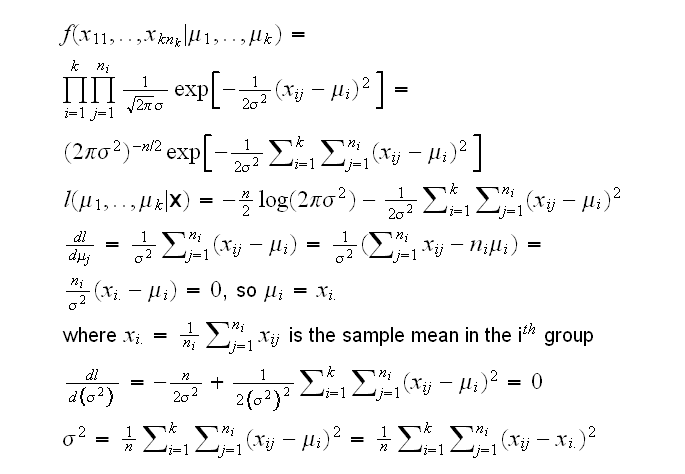
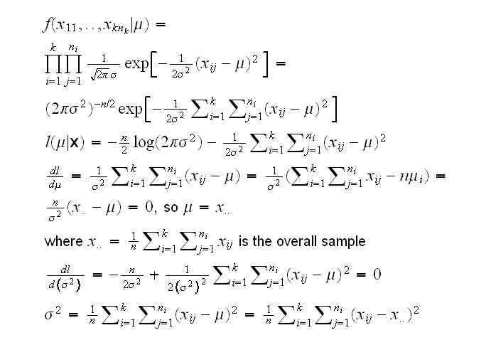
Let's derive the likelihood ratio test for this problem:
under the null hypothesis μ1=...=μk=μ and so
Let's call the estimate of variance under the null hypothesis s02, and under the alternative s12, then
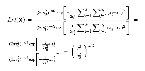
you can now see why this is called the analysis of variance although it really is a method concerned with means. Now
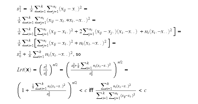
In the numerator we have an estimate of the variance between the group means and the overall mean, and in the numerator an estimate of the variance within the groups. It is easy to show that this test statistic (when properly scaled) has an F distribution with k-1 and n-k degrees of freedom.
Let's find all the relevant numbers for our dataset:
x..=49.55 (overall mean)
x1.=51.1, x2.=49.3, x3.=48.0
so ∑ni(xi.-x..)2 = 39(51.1-49.55)2+19(49.3-49.55)2+36(48.0-49.55)2 =181.375
∑i∑j(xij-xi.)2=885.58
Next we find the mean squares by dividing each with its degrees of freedom: 181.375/2=90.69, 885.58/91=9.73
then we find the F-statistic as the ratio of the mean squares 90.69/9.73=9.31
and finally the p-value=1-pf(9,31,2,91)=0.0002
now the information is usually summarized in an ANOVA table:
| df | sum of squares | Mean Square | F value | p-value | |
|---|---|---|---|---|---|
| Status | 2 | 181.375 | 90.69 | 9.318 | 0.002 |
| Residuals | 91 | 885.58 | 9.73 |
The basic F test is rarely of great interest, ANOVA becomes more interesting when we test more specific hypotheses.
A contrast is an expression of the form ∑aiμi where (a1,..,ak) is such that ∑ai=0. With this notation we can write many interesting hypotheses:
• basic F test: H0: ∑aiμi =0 for all (a1,..,ak) is such that ∑ai=0
• multiple comparison test: H0: ∑aiμi =0 for (1,-1,0) (1,0,-1) and (0,1,-1)
• a test of interest in a specific situation: H0: ∑aiμi =0 for (1/2,1/2,1) tests whether (μ1+μ2)/2=μ3
To test H0: ∑aiμi=0 vs Ha: ∑aiμi≠0 use the Test Statistic

Example for the cocain data test whether there is a difference between the Trimester and the Throughout groups.
we have
H0: ∑aiμi =0 vs Ha: ∑aiμi ≠0 for a=(0,1,-1)
so

One important point to remember here is that the classical ANOVA method is "just" a straightforward application of the likelihood ratio test.
This will of course always depend on the priors on (μ1,..,μk,σ). If we choose noninfomative priors, for example proportional to 1/σ2, then we recover essentially the classical ANOVA above.